You may have noticed in the last few labs that while we can control bring our system under control, the ability of it to "track" (approach the input value in steady state) exactly what we want (our input) isn't amazing. In particular, as we go further and further away from a horizontal arm position, things gets worse and worse.
Now, we're certainly trying to improve tracking in things we do. That pre-compensator gain, \(K_u\) which we've shown to be: \[ K_u = \left(\textbf{C}\left(\textbf{I}-\textbf{A}+\textbf{BK}\right)^{-1}\textbf{B}\right)^{-1} \] ...and which we've shoved into the our system's input is an effort at improving tracking, and it does help. Without the precompensator gain, your system's ability to track the input is even worse.
Are there other ways to improve our system's ability to track the input? While the movement of the eigenvalues/natural frequencies that we've focussed on in weeks 1 through 3 can be thought of as a means of getting our system to converge to an output and do so quickly and reliably, we haven't done much else to improve what our system converges to.
Much of this comes down to the famous statement said by somebody, "All models are wrong, but some models are useful." The model that we've been basing all of our state space thinking and calculations around isn't perfect, and while a physics-based model isn't a bad way to go about designing and or controlling a system, sometimes it won't be enough. In Week 4 we're going to look at two different methods for dealing with our less-than-perfect model and how it pertains to the tracking error it introduces. In the first part, we're going to move back to full-state feedback from Labs 1 and 2, but add an additional state to our state space model that contains the integral of error. This is somewhat similar to the "I" term in "PID" control from 6.302.0x, but when in state space form a bit more thought/math needs to be dealt with to properly deploy this term.
In the second, more experimental section, we're going to just resign ourselves to not knowing what the physics of our system are and instead, using a frequency sweep, we'll generate and construct a "grey-box" model of our system upon which we'll create and use an observer.
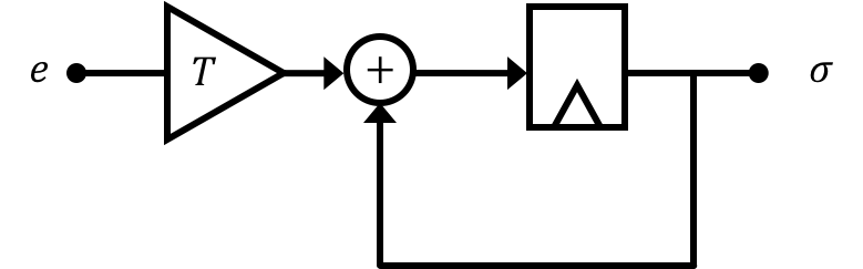
We've already seen integration a number of times here. In a discrete time block diagram, the act of integration will generally take the following form:
If we base our system response just on the error (relationship of output to commanded input) in a system (and also with its discrete time derivative (see 6.302.0x)), we can generally get it to stabilize. We're doing that here in 6.302.1x just from a different, more generalized perspective via matrices and states. With this, however the system can eventually reach a stable configuration where it may "tolerate" a steady-state error. If however, we integrate/accumulate error over time we obtain another means of responding to error. It gives the system the ability to start seeing a certain amount of error as less and less tolerable as time goes on (since the integral of that error will grow as time goes on).
In this lab we're going to introduce a new state called the error integral. At first glance this state might seem less "physical" than some of the other system states like velocity, angle, etc., but it is still just as valid. Think of an integral state as a timer that starts counting up or down based on the value and magnitude of an error. The shot clock in basketball or similar timing mechanisms in many other sports are all similar to an error integral state (although in basketball it is highly thresholded and discretized so not what we'd call LTI, it is still integrating the position of a player, for example).
Let's start off by creating a variable for the error of our system \(e[n] = y[n] - u_d[n]\) where \(y[n]\) is our output and \(u_d[n]\) is our pre-compensator input. Let's then come up with an expression for the discrete time integral (or what we could call the accumulation of error). We'll call this term \(\sigma\) and say that: \[ \sigma[n] = \sigma[n-1] + Te[n-1] \]
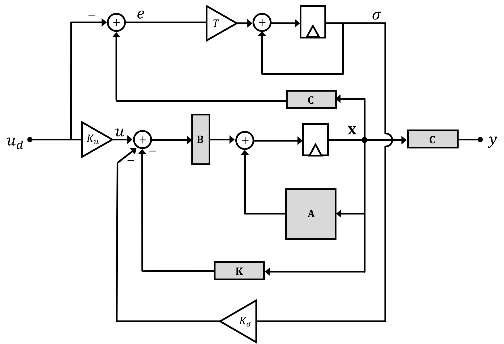
Remembering that \(y[n] = \textbf{C}\textbf{x}[n]\) in our state space system we could then say: \[ \sigma[n] = \sigma[n-1] + T\left(\textbf{C}\textbf{x}[n-1] - u_d[n-1]\right) \] When we integrate (pun definitely intended) this new variable into our original open loop state space system diagram we'll end up with the following:
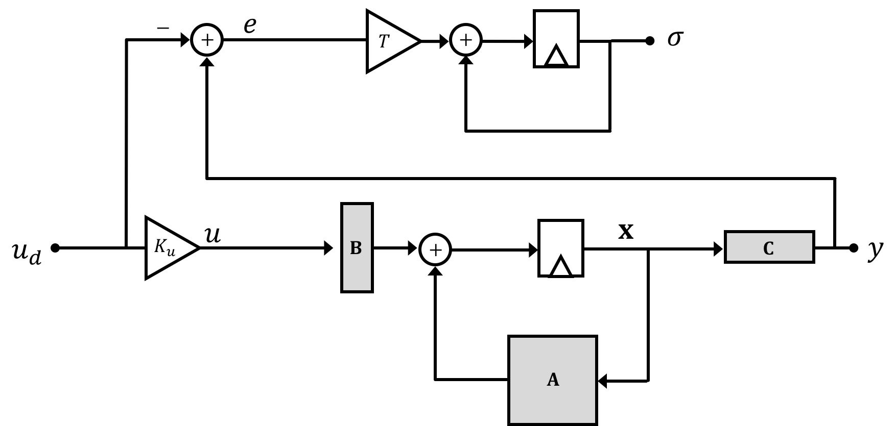
We're drawing the system diagram in this weird way for a reason that will become apparent in a moment. But for right now if we merge our general state space system equation with the difference equation we've generated for the integral of error \(\sigma\) we get: \[ \begin{bmatrix}\textbf{x}[n+1]\\\sigma[n+1]\\\end{bmatrix} = \begin{bmatrix}\textbf{A}& 0\\T\textbf{C} & 1\end{bmatrix}\begin{bmatrix}\textbf{x}[n]\\\sigma[n]\\\end{bmatrix} + \begin{bmatrix}\textbf{B}\\0\end{bmatrix}K_uu_d[n] + \begin{bmatrix}\textbf{0}\\-T\end{bmatrix}u_d[n] \] Now this new set of equations itself takes on the same "shape" as any general state space equation so we can lump stuff together to generate a new set of equations and terms. Graphically this "lumping together" looks like the following where we denote our new matrices that include the integral term with a tilde on top (\(\tilde{~}\)).:
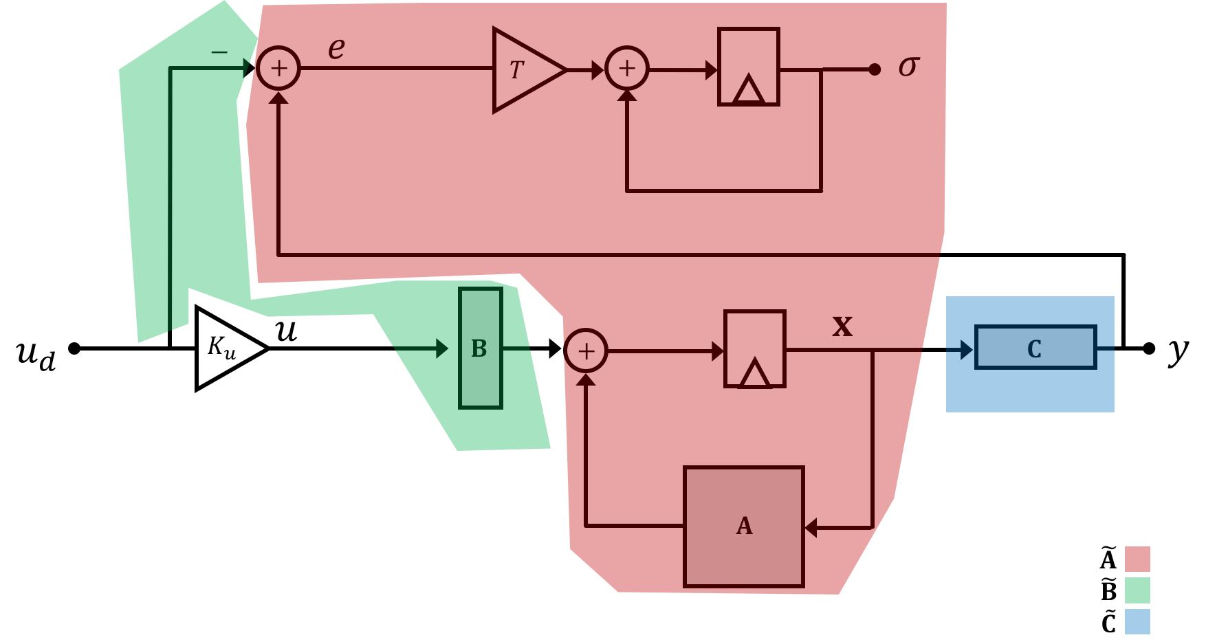
and we'll have two state space equations: \[ \tilde{\textbf{x}}[n+1] = \tilde{\textbf{A}}\tilde{\textbf{x}}[n] +\tilde{\textbf{B}}K_uu_d[n] \] and \[ y[n] = \tilde{\textbf{C}}\tilde{\textbf{x}}[n] \] where: \[ \tilde{\textbf{x}} = \begin{bmatrix}\textbf{x}\\\sigma\end{bmatrix} \] \[ \tilde{\textbf{A}} = \begin{bmatrix}\textbf{A} & 0\\T\textbf{C} & 1\end{bmatrix} \] \[ \tilde{\textbf{B}} = \begin{bmatrix}\textbf{B} \\ \frac{-T}{K_u}\end{bmatrix} \] \[ \tilde{\textbf{C}} = \begin{bmatrix}\textbf{C} & 0\end{bmatrix} \] And so we can redraw the entire system in this form:
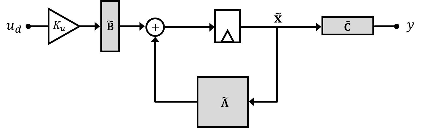
The integrator state \(\sigma\) has now lengthened the state vector from its initial value of \(m\) to \(m+1\). This means that all the other matrices have adjusted accordingly with \(\textbf{A}\) going to \(m+1 \times m+1\), \(\textbf{B}\) going to \(m+1\times 1\), \(\textbf{C}\) going to \(1 \times m+1\) and \(\textbf{D}\) staying at \(0\) (for our class anyways). Importantly, along with that new state will come another eigenvalue!
Another thing to keep in mind is that error uses that value of input before the pre-compensator \(K_u\). It isn't a big deal here, but it will cause potential headaches in the next part so be on guard!
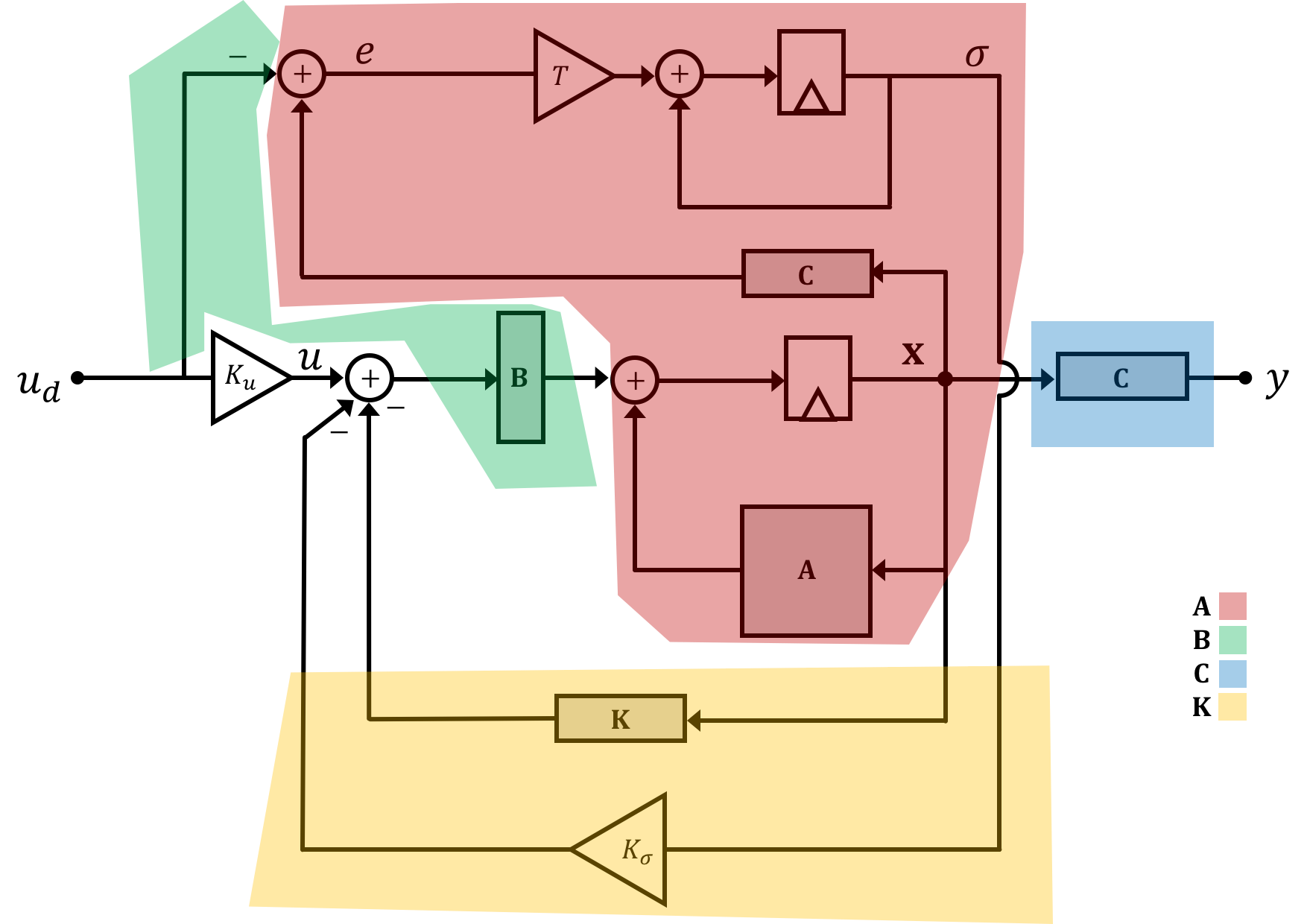
OK we now have our new open loop system with our modified matrices that include the error integral state in them. Like all of our state space systems, we will probably want to put this into feedback to adjust the natural frequencies/eigenvalues of the system, but instead of doing this as we've already learned, we're going to stick with the un-lumped system for the moment as drawn below.
Few things to note below: the \(\textbf{C}\) matrix has been duplicated to simplify the drawing. These are still the same exact matrix and we could have the output signal coming back from the terminal labeled \(y\) explicitely but I wanted to minimize wires crossing.
Secondly as drawn \(\textbf{K}\) is still our standard gain vector from before (of original size too!). \(K_{\sigma}\) is a scalar gain value applied only to the error integral signal.
Similar to the open loop system above, we can derive a new set of equations describing this whole system: \[ \begin{bmatrix}\textbf{x}[n+1]\\\sigma[n+1]\\\end{bmatrix} = \begin{bmatrix}\textbf{A}-\textbf{BK} & -\textbf{B}K_{\sigma}\\T\textbf{C} & 1\end{bmatrix}\begin{bmatrix}\textbf{x}[n]\\\sigma[n]\\\end{bmatrix} + \begin{bmatrix}\textbf{B}\\0\end{bmatrix}K_uu_d[n] + \begin{bmatrix}\textbf{0}\\-T\end{bmatrix}u_d[n] \]
And just like above we can lump parts of this expression together:

It seems that adding the integral term in wasn't too bad. We've now come up with an expression for our system matrix \(\textbf{M}\) as modified by full state feedback!. Fantastic. As we'll remember from Week 2, if a system is controllable (they are for our class), you can request any set of desired natural frequencies and calculate (either analytically or numerically) a set of gain values to achieve this.
We've been using Ackermann's Method to do this, which we've used like the following:
des_nat_freq = [0.999,0.999,0.999]
k_acker = acker(A,B,des_nat_freq)
We would then use the values in k_acker for our gain vector \(\textbf{K}\). In the case of our system that includes an integral, we'll want solve for \(\tilde{\textbf{K}}\) where
\[
\tilde{\textbf{K}} = \begin{bmatrix}\textbf{K}\\K_{\sigma}\end{bmatrix}
\]
Should we just put in our \(\tilde{\textbf{A}}\) and \(\tilde{\textbf{B}}\) matrices which we solved for eariler on? Not necessarily and this is because our error is based on a pre-\(K_u\) value which tangles up some of our math. What acker is expecting is a set of "A" and "B" matrices that fit the following shape: \(\textbf{M} = \textbf{A}_f-\textbf{B}_f\textbf{K}_f\) which in our particular case looks like the following:
\[
\begin{bmatrix}\textbf{A}-\textbf{BK} & -\textbf{B}K_{\sigma}\\T\textbf{C} & 1\end{bmatrix} = \textbf{A}_{f} - \textbf{B}_{f}\tilde{\textbf{K}}
\]
What \(\textbf{A}_f\) and \(\textbf{B}_f\) matrices satisfy this equation for us?
\(\textbf{A}_f\):
\(\textbf{B}_f\):
So using the matrices determined above, we now know how we can pick our system feedback gains with an integral term included! The same rules/thought processes apply in terms of what are good and bad natural frequencies to ask for (see week 2), just remember that instead of asking for \(m\) natural frequencies (where \(m\) is the number of states in your original system), you should now be asking for \(m+1\) because of our added integral state!
The next question comes from calculating our precompensator gain \(K_u\). If you remember from Week 1 and 2, we calculate this value after our feedback gains are calculated. How does the appearance of this new state affect our \(K_u\) calculation therefore? We'll discuss on the next page.
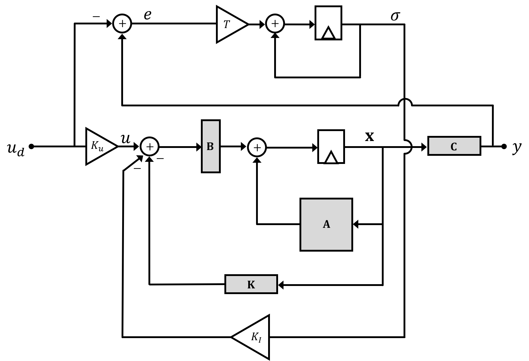
On this page we'll figure out what the precompensator gain \(K_u\) should be when we have an integrator state added into the mix. Like on the previous page where the fact that error is based on the pre-precompensator signal, it will also mess cause some problems from that may not be apparent if we "hide" our new integral state inside the new state vector. So first let's remember our overall system diagram with an integrator in it. We'll keep the integrator state \(\sigma\) separated from the original system states for the purposes of this derivation:
Just like in week 1, determination of an expression and/or value for \(K_u\) is a relatively easy derivation. If we assume the system can reach a steady-state value (that is that we can modify its natural frequencies via feedback to have it converge on a stable set of states), when the system reaches steady state we can say that \(\textbf{x}[n+1] = \textbf{x}[n]=\textbf{x}[n_{\infty}]\) where we use the subscript \(\infty\) to represent timesteps far in the future after the system has stabilized (very large \(n\) or as \(n\to \infty\)). This is basically saying that from time step to time step the states will not be changing, which if we're dealing with a constant input (relative to system dynamics) is exactly what we want. This holds for all the system's values including our integral signal \(\sigma\) where \[ \sigma[n] = \sigma[n-1]+Te[n-1] \] where we say \(e[n] = y[n] - u_d[n]\). Now just like everything else in the stable system which converges at large \(n\) we can say that \(\sigma[n] \approx \sigma[n-1] = \sigma[n_{\infty}]\). This implies, therefore that at steady state, \[ Te[n-1] = 0 \] This in itself is a neat conclusion to draw. If we can stabilize our system and have all of its states converge to steady state values that implies that the error of our system at steady state must go to zero! Very nice and exactly what we want!
The question still remains, as to what value \(K_u\) should be set. Let's jump back to our full state space expression where we stack the integral in with our original state vector. If the system converges then at very large \(n\) we can assume: \[ \begin{bmatrix}\textbf{x}[n_{\infty}]\\\sigma[n_{\infty}]\\\end{bmatrix} = \begin{bmatrix}\textbf{A}-\textbf{BK} & -\textbf{B}K_{\sigma}\\T\textbf{C} & 1\end{bmatrix}\begin{bmatrix}\textbf{x}[n_{\infty}]\\\sigma[n_{\infty}]\\\end{bmatrix} + \begin{bmatrix}\textbf{B}\\0\end{bmatrix}K_uu_d[n_{\infty}] + \begin{bmatrix}\textbf{0}\\-T\end{bmatrix}u_d[n_{\infty}] \] We can shuffle this to: \[ \left(\textbf{I} -\begin{bmatrix}\textbf{A}-\textbf{BK} & -\textbf{B}K_{\sigma}\\T\textbf{C} & 1\end{bmatrix}\right)\begin{bmatrix}\textbf{x}[n_{\infty}]\\\sigma[n_{\infty}]\\\end{bmatrix} = \begin{bmatrix}\textbf{B}K_u\\-T\end{bmatrix}u_d[n_{\infty}] \] and then: \[ \begin{bmatrix}\textbf{x}[n_{\infty}]\\\sigma[n_{\infty}]\\\end{bmatrix} = \left(\textbf{I} -\begin{bmatrix}\textbf{A}-\textbf{BK} & -\textbf{B}K_{\sigma}\\T\textbf{C} & 1\end{bmatrix}\right)^{-1} \begin{bmatrix}\textbf{B}K_u\\-T\end{bmatrix}u_d[n_{\infty}] \] and then since \(y[n_{\infty}] = \tilde{\textbf{C}}\begin{bmatrix}\textbf{x}[n_{\infty}]\\\sigma[n_{\infty}]\end{bmatrix}\) we can say: \[ y[n_{\infty}] = \tilde{\textbf{C}}\left(\textbf{I} -\begin{bmatrix}\textbf{A}-\textbf{BK} & -\textbf{B}K_{\sigma}\\T\textbf{C} & 1\end{bmatrix}\right)^{-1} \begin{bmatrix}\textbf{B}K_u\\-T\end{bmatrix}u_d[n_{\infty}] \] and then....we'll we're sort of stuck. This is expression is not really useful to our needs of isolating \(K_u\) and in fact, we'll end up with infinite solutions to this problem which isn't really helpful.
As an alternative, we can try to assume that if we pick a good \(K_u\) and the system is operating in a controllable sense, long-term the system's integral of error should be close to zero so we can ignore our integral term in this expression. If that is the case then we can then fall back to our starting equation which then becomes: \[ \textbf{x}[n_{\infty}] = \left(\textbf{A}-\textbf{B}\cdot\textbf{K}\right)\textbf{x}[n_{\infty}] + \textbf{B}K_uu_d[n_{\infty}] \] This is exactly the same setup as before actually from week 1! This can eventually be derived to show that under this assumption the expression for \(K_u\) is: \[ K_u = \left(\textbf{C}\left(\textbf{I}-\textbf{A}+\textbf{BK}\right)^{-1}\textbf{B}\right)^{-1} \]
Notice that in this derivation for \(K_u\) we are using the original state space matrices and vectors and not the modified ones such as \(\tilde{\textbf{A}}\)! This is important! When calculating \(K_u\) in the case of an integral, you should use your original matrices and not the "newer" ones!
Now that we've cleared up some math, most of what we're doing for the lab is to implement the integral control. This will involve two files that are mostly completed for you (although feel free to change and experiment with them how you want). There is a PYTHON FILE and a MICROCONTROLLER FILE. Download both.
The Python code is an expansion of Week 2's code. Follow along with the comments in the file. From our original 3-state model (included here), we build up a four state model (where the fourth state is the integral term). We then proceed to carry out the gain selection and system construction for both the original 3-state model and the four state model. At the bottom, the four state system output is plotted. Feel free to plot both and compare. As before, iterate through using this code to generate a set of gains and then implement them on your system below. You don't need to hard-code anything thin the microcontroller for this lab, so feel free to keep the system running and try different gains in real time!
The code for the Teensy is almost unchanged from what was used in Lab 02. Modifications include:
intV which is used to store the integral state within and between loop iterations.Integral states are often subject to what is known as "Integral Windup" where in certain situations too much integral can build up resulting in a massive compensation effect. This will most likely happen in our setup when the power isn't turned on but the system is running. To limit this to a certain extent we clip the integral term when it goes above or below a certain range to prevent the windup from going too far. This is often done in PID controllers as well The following code shows how we do that:
//Calculate Integral:
intV = intV - errorV*dTsec; //error is y - u_d so minus here

if (intV>=integralMax){
  intV = integralMax;
}else if(intV<-1*integralMax){
  intV = -integralMax;
}
The microcontroller code should just run as is...although of course always feel free to change if you want.
With these sets of code, you should be able to determine a set of gains that control the system with an integral control added in. You will probably find the dynamic response of the system somewhat poorer with the integral than without the integral, but tracking will be improved. Test this and see. One reason for this is that where our three state model has the following open-loop natural frequencies:
1.0000 +2.8798e-07j, 1.0000 -2.8798e-07j, 0.9944 +0.0000e+00jOur four-state open loop model has the four natural frequencies:
1.0000 +5.3383e-05j, 1.0000 -5.3383e-05j, 0.9999 +0.0000e+00j, 0.9944 +0.0000e+00j
This new set is not an easier starting position...in fact it is worse...we still have two complex natural frequencies outside the unit circle and one just on the inside. But now we have a fourth one also just on the inside at a not particularly good location. The more natural frequencies that we need to move inward, the more "work" will be needed to do this (where "work" implies either more time or higher values of states and input to make it happen quickly). So basically this integrator has come with a cost.
Another issue that will start to come to light in this lab is that the pole placement mechanism given to use by acker may start to less satisfying that before. All acker does is provide four gains that move the natural frequencies appropriately, and then we as humans have to watch what it produces and adjust accordingly based on state values and other things it specifies. With acker there's almost no ability to specify which states we're more or less ok with having high values, however. Everything is sort of black-boxed together. A different approach to this problem (LQR) is detailed in notes that have also just come out on the site. LQR, while more difficult to set up, provides more flexibility in terms of stating what states we're ok with going to high temporary values. Consider trying to implement LQR control in this lab to see if you gain any more flexibility)
So far in this course our propeller control and the various flavors of it have been built around a state space model we derived from physical principles in Week 1. This model used theory and what we as a human society have learned about the universe over the past few millenia to create a set of relationships between system parameters which we assembled into a system of equations, which we then thought of as matrices and went from there.
We did make a lot of assumptions in creating that model, however, and even the model on its own wasn't enough to generate proper control. We had to add in that "directV" term to offset gravity and do some other tricks like linearization of a highly quadratic phenomenon. The parameters we used for our system model were derived in conditions slightly different from how we run our propeller (and they were derived for my propeller...not yours...and chances are that at this price point, these are not manufactured to obsessive precision/consistency so variation should be expected.
One Solution to this is to rely more on data taken from the exact system and that's what we'll do in this lab. First we're going to stabilize our system using Proportional + Derivative control that we used/studied in 6.302.0x. We'll then stimulate this stabilized system with a bunch of sine waves of known frequency and amplitude, and measure the phase and magnitude difference of the resulting sine wave signals before (our command signal) and after (the arm angle) our plant and use the resulting magnitude and phase differences to extract a model. In the process of doing this, everything that goes into making our plant what it is can potentiall be captured...not just our simple physics equations and abstractions. The idea is to then more
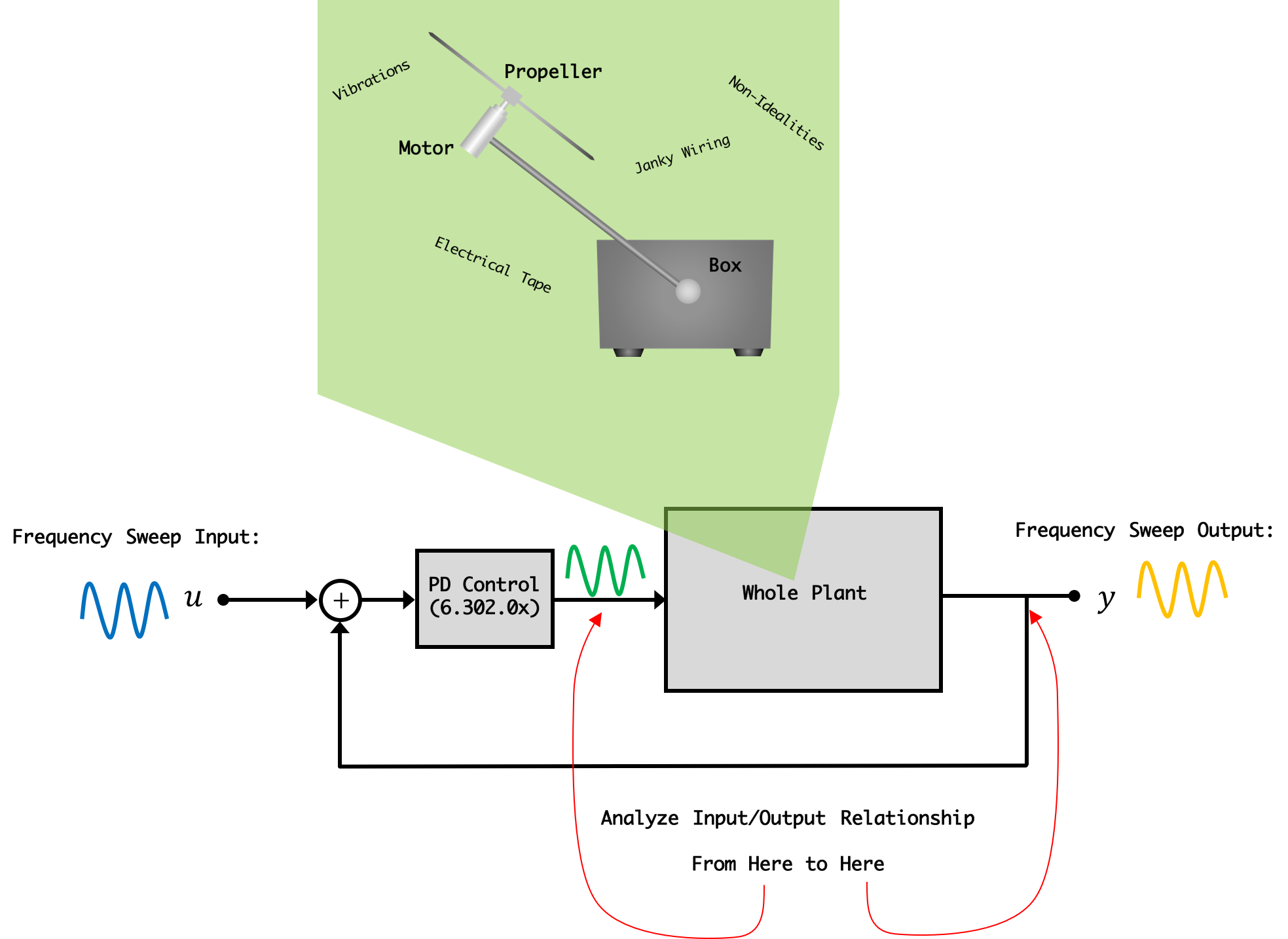
The term "grey box" modeling is sort of a play on the more common term "black box" where a black box refers to a system of which we have no idea of the inner workings...only its inputs and outputs. A black box model is purely input-output data-based....it is a black box; we can't see inside it. In grey-box modeling we use some physical intuition and ideas to help guide a data-driven model and we'll do that in this lab.
There won't be much "math" or derivations in this lab. Instead we're just going to be applying a lot of the concepts we've already touched upon with different data sets to hopefuly get a better-performing system!
There are THREE pieces of code for this lab and discussion of their functionality serves as a good outline of what we need to do:
The files will generally be used in the order listed above
This code is a frequency sweeper that uses Proportional+Difference Control for stabilization (from 6.302.0x). It inputs sine waves of various frequencies and analyzes the amplitude and phase of the resulting sine waves of the "command" signal and the output of the system. These values are recorded in a CSV file (if you tell it to do that which you should!) There should be only one line you need to change in this code: Line 148:
//Need to change for your system!!!
float directV = 1.4;
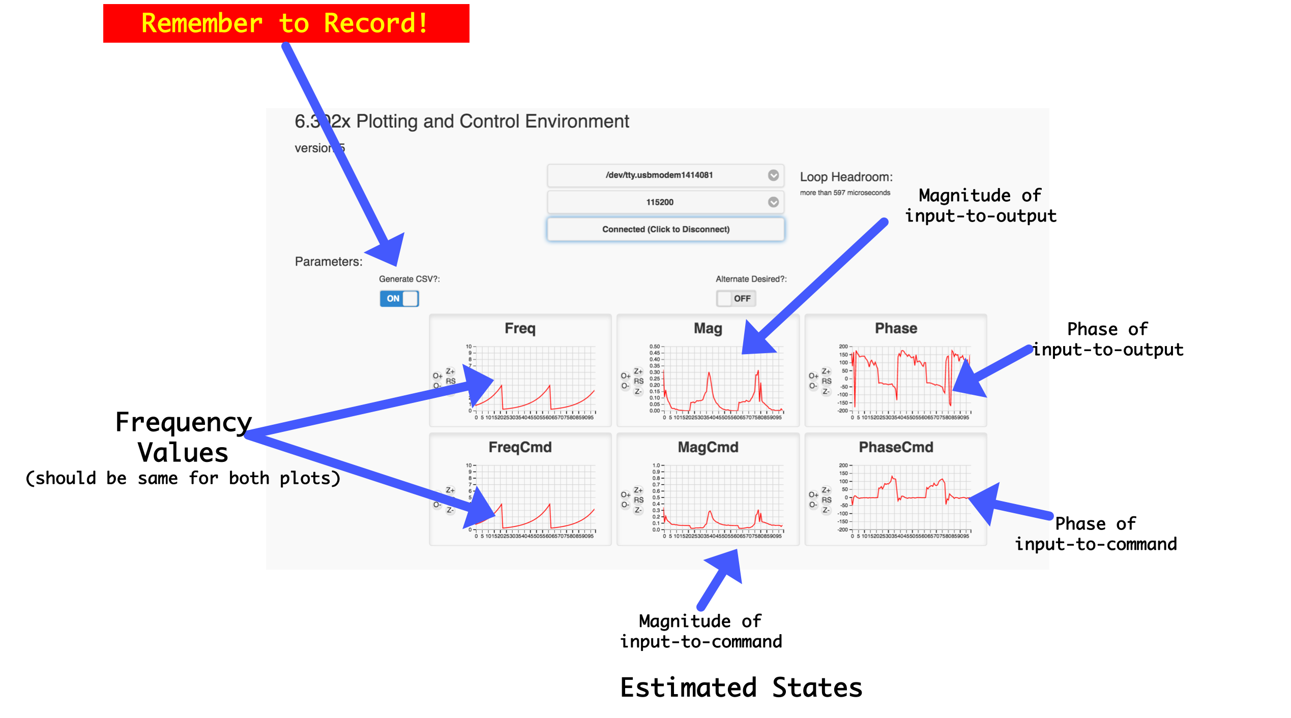
This is the direct term you need to roughly "level" your system's arm. 1.4V is generally what it has been for my setup, but your's will vary depending on motor, type/length of arm, etc... Once you've made this change, upload this code, start the server.py, and connect via the GUI. the system will immediately start running so help it get to level if it doesn't do it on its own. Once it seems to be running fine, turn on the "Generate CSV" button (VERY IMPORTANT...without it you don't generate data), and let it run. This system will take ~2 minutes to run one full data-collection cycle (sweep through all frequencies). We encourage you to let it run at least three cycles to let us hopefully filter out noise/bad measurements (averaging of readings takes place in the Python file below.)
While running your plots should look like the following:
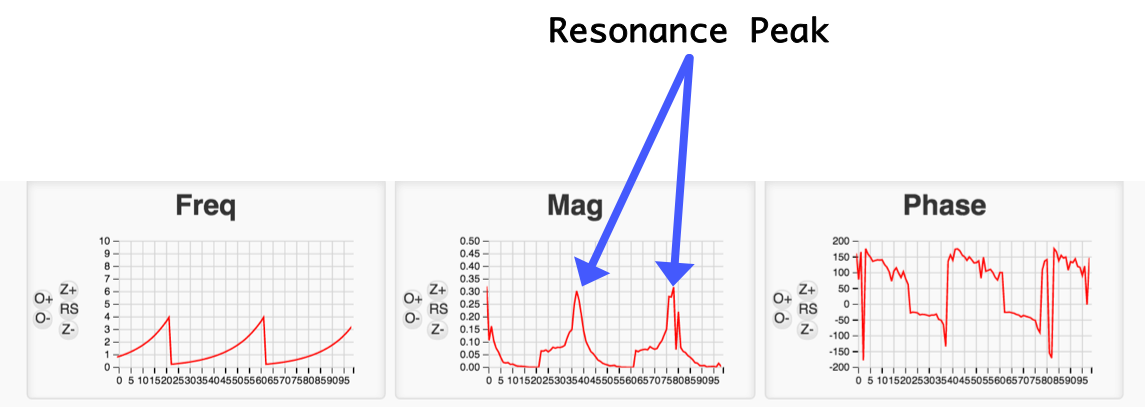
For at least the first couple times, it is good to sit and watch your system. While sweeping the system will most likely hit resonance, where you're stimulating it with frequencies close to or at your system's natural complex frequencies. If your system is too resonant, you should slightly back down the amplitude term in line ~146 in your code:
//angleV = 0;
float angleVdesired = 0.15*sinv;
A sharp resonance peak is a really useful feature to extract for model building so we don't want to back this amplitude down too much, but too much resonance will be too much for our PD control to stabilize and can cause your system to oscillate past the vertical and get stuck! For example when I bump up
angleVdesired on my setup to about 0.18, my system loses control at its resonance peak! I found 0.15 is a good starting value. If you do need to change this value, you'll need to reupload your code and start again.
Once your system is running reliably, let it take a bunch of data cycles (really the more the better), so leaving the GUI window up, go have a coffee or tea or meditate or watch an episode of Halt and Catch Fire (season 1...season 2 gets not as good). When done, go ahead and stop recording your data. Your ready to move onto the next part (Model Extraction).
To use this file, move/rename(if you want) the csv file corresponding to a good data set from your frequency sweep. If this is the most recent data set you took it will be known as both current.csv and timestamp.csv where timestamp is the epoch time of when the file was written (seconds since Jan 1, 1970).
Feel free to dig through the file and read the comments and ask questions about it in the forum, but in general the only thing you should need to change in the file are the name of the csv file you want to extract data from, and the set of plant and observer natural frequencies (using variables similar to Lab 03's code).
If you run this and no errors pop up you should get a readout detailing the extracted model and some other things. For example for one of my data sets I got the following information printed out:
coefficients found:
(array([ 35.9537,   7.3999,  25.8108,   2.904 ]), 1)
State Space Model Generated:
A = [[  9.9709e-01  -2.5777e-02  -7.3891e-03]
 [  9.9855e-04   9.9999e-01  -3.6964e-06]
 [  4.9952e-07   1.0000e-03   1.0000e+00]]

B = [[  9.9855e-04]
 [  4.9952e-07]
 [  1.6655e-10]]

C = [[  0.       0.      35.9537]]

D = [[ 0.]]

dt = 0.001

Eigenvalues of State Space Model:
[ 0.9987+0.0048j  0.9987-0.0048j  0.9997+0.j    ]
#K Gains for requested plant natural frequencies:
[[  26.9768  273.6203  994.055 ]]
L Gains for requested observer natural frequencies:
[[ 0.4946]
 [ 0.067 ]
 [ 0.0024]]
Ku Value: 27.8540
You'll use the model generated and the gains you pick for implementing observer control of your system in the next section!
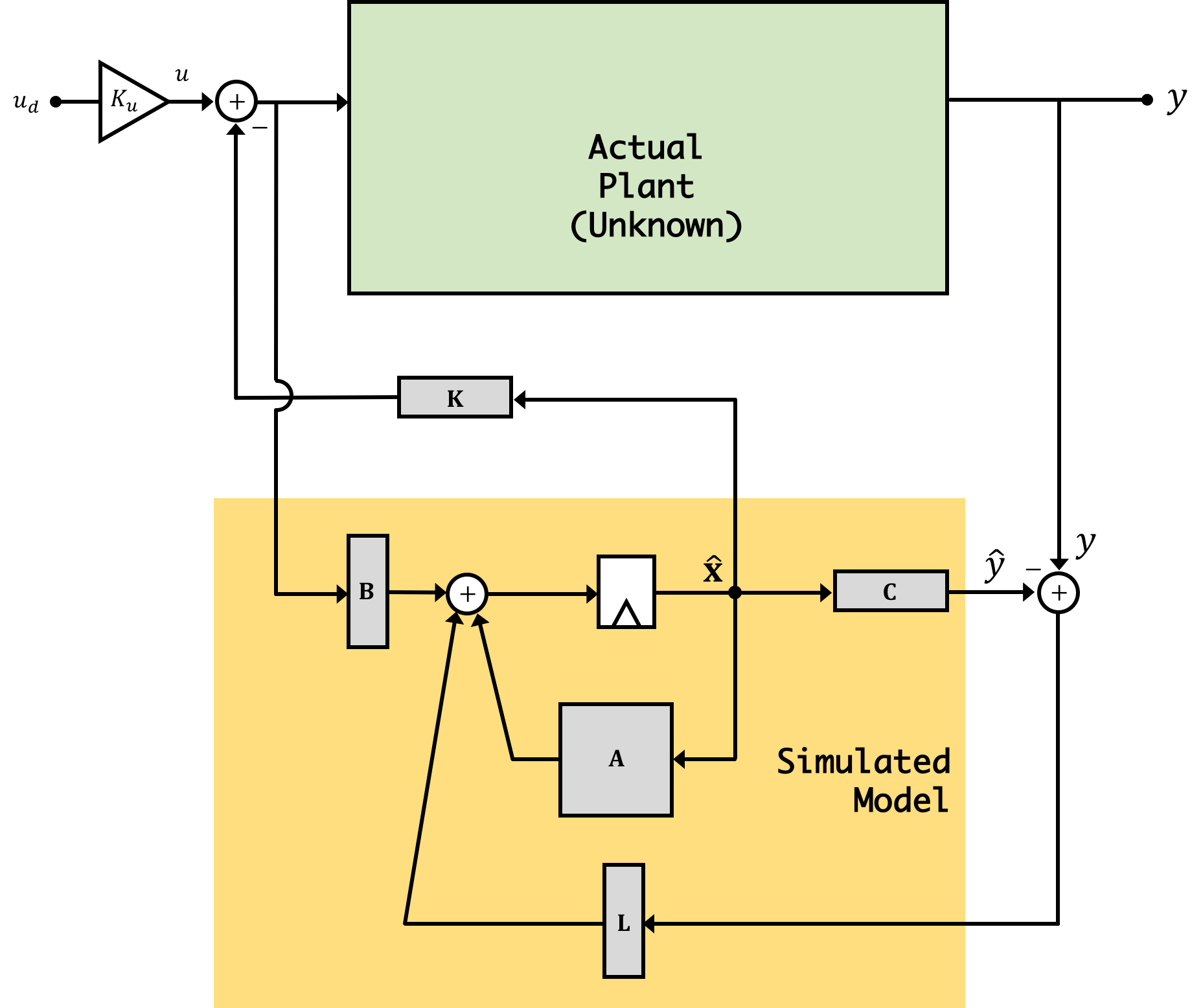
The last piece of code in this workflow is a three-state observer-based controller (very similar to Lab 03). Just like in Lab 03, you need to fill in the parameters for your system model (\(\textbf{A}\), \(\textbf{B}\), and \(\textbf{C}\) matrices, your feedback gains \(\textbf{K}\), and your obserer gains \(\textbf{L}\). This time, however you're going to use the extracted values that pop out of your Python file.
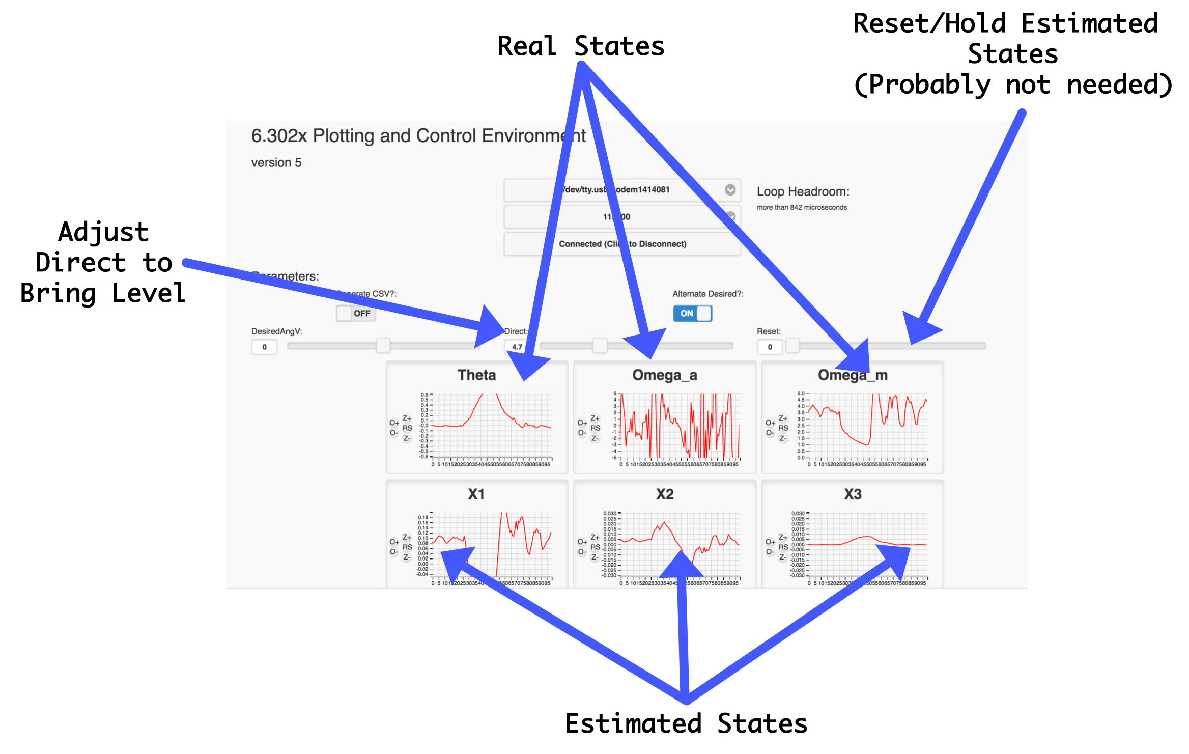
Once you've done this, upload to your microcontroller, and get it running! Upon startup you should see the system probably start moving a little, but you'll need to bring in a direct term as before to get it working. The GUI will plot six things for you: The three "real" states, and the three states generated in your model. These two groups may not correspond to eachother one-to-one. For example, in some of my data sets found that in my extracted model my state 3 was about proportional to what my angle was but that my states 1 and 2 were somewhat a mix of both back EMF and angle derivative.
The code overview on the previous page should have given a basic outline of what you need to do in this lab. Like all of our labs, however, this one will involve iterations so be prepared to take multiple frequency sweep data sets and generate different models and apply them and go back and forth. This is how engineering and design is. Very rarely is a design process linear.
Be willing to experiment with different settings. For example, see if you generate a different model for your system if you adjust direct so that the arm is slightly below or above the horizon. I found more resonance when below and less when above, for example, and this gave me different models each time. The model for the below-horizon plant was significantly less useful when I then went and applied it above the horizon.
Experimentation with different plant and observer gains is also a good direction to go here and one in which you probably will have to go in order to get your system working. You could also consider adding in an integral term with your observer or using LQR instead of acker to arrive at controller and observer gains! There's really a lot of different directions to take this lab.
Both Jacob and I (as well as a number of residential students), got by-far the best control we've yet obtained via this grey-box approach, and this should make some sense...we're building a model off of the system itself not our abstraction of the system. We'd like to emphasize that building a model this way doesn't invalidate our previous approaches and what we've discussed. We're still using everything we've discussed in this lab. And the "grey" part of our grey box modeling is relying on things which we've tested and validated in previous labs. For example, we use the fact that the system can be reliably modeled and controlled with a three-state model to know what to fit our data too for example. Also we wouldn't know how to implement an observer if it weren't for previous state space techniques. Sometimes we don't have the luxury of collecting data on a system like we do here, and therefore models are all one may have to go off of.
The fitter code we are using in the Python file here is not very robust so if you generate particularly bad frequency data from your sweep, the fitter may have trouble converging or it may converge to something that doesn't make much sense. Signs of bad fitting include a large negative number in the first value of the coefficients found array. If you've got access to MATLAB and its control systems package, they have a fantastic tool called tfest that is really impressive and does way better than the basic least-squares fitter we have here. If you're interested in messing with it, we have a matlab script we can provide...but that requires MATLAB to use.