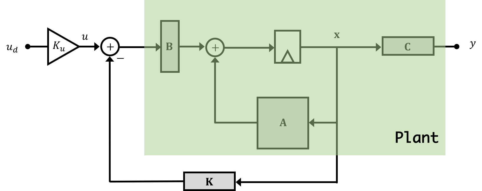
In the last two weeks we've discussed the benefits and some very basic techniques for designing state space controllers. So far this has generally involved:
This can be a pretty reliable way of going about designing and controlling state space systems, however it is making one major assumption: that we have access to all of the system's states. To understand what is meant by this consider our anesthesia problem from Week 02. There are a number of states in this model, which can be thought of as modeling different biological membranes/barriers/transfers in the body (lung-to-blood, blood circulation, blood-to-brain, etc...). The "meaning" of these states could then be thought of as the lecurrent rate of anesthetic compound moving through those different barriers at different points in time:
Now if we pause and think about the amount of equipment and sensors needed to actually get at that information in real-time, you'll quickly recognize that full-state feedback as presented, while nice sounding would be way too invasive to properly implement on a person. In addition are questions about instrumentation...how would you even measure the transfer rate of anesthetic compound through the blood-brain barrier in real time? The answer is you wouldn't and this happens a lot in state space control. There are often numerous states in system models that we come up with that cannot, because of a lack of practicality (financially, physically, etc...), be measured. So while we might want the top system below, the bottom system is sometimes what we have to deal with
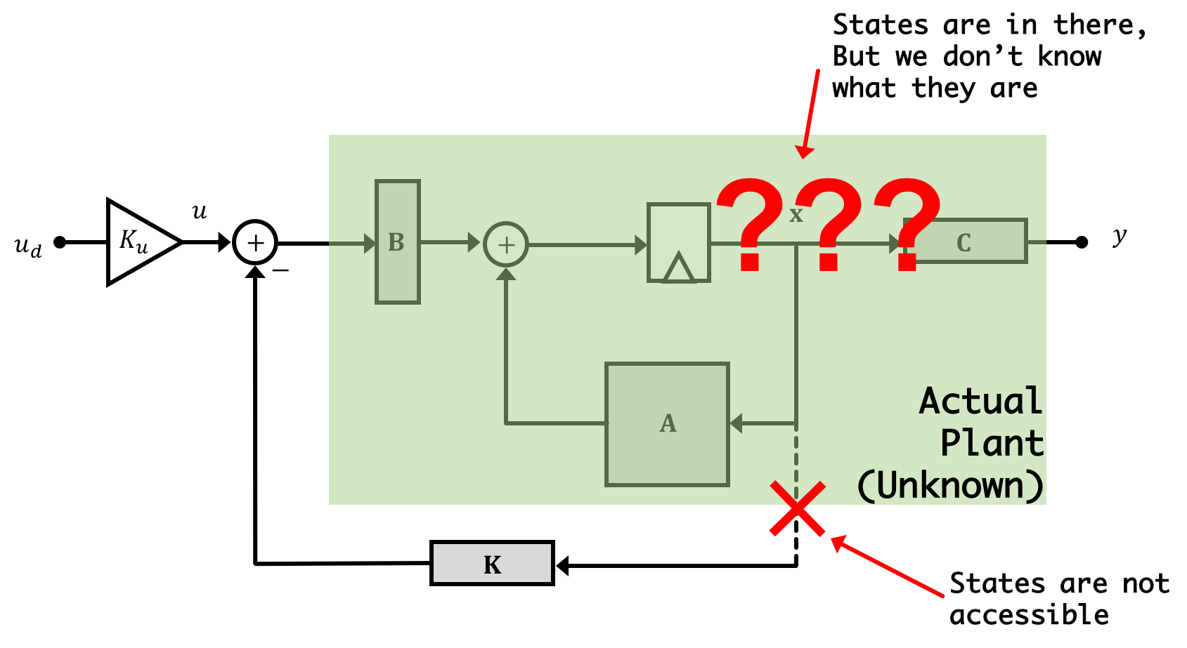
What do we do? The solution is Observers!
An observer is model that we simulate of our system in real-time (so it will be done on the microcontroller at run-time). The observer is a state space system in its own right, so it has states and we'll want to avoid confusing them with the states of the real system. In order to distinguish its states (the simulated states) from the actual states of the real plant, we're going to denote them with a "hat" so that the observer's state vector will be \(\hat{\textbf{x}}[n]\). Similarly we'll say the output of the observer is \(\hat{y}\) to distinguish it from the output of the actual plant \(y\).
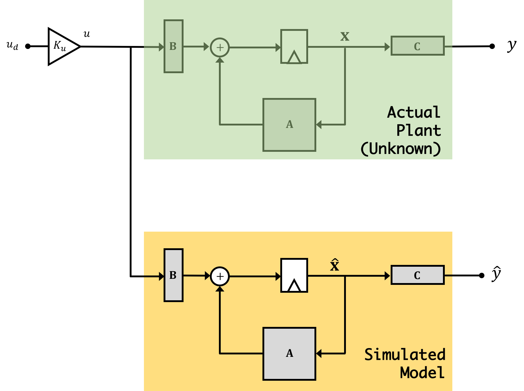
As stated above, the observer is a full-on state space system so it can be described by its own set of state space equations like that shown below: \[ \hat{\textbf{x}}[n+1] = \textbf{A}\hat{\textbf{x}}[n] + \textbf{B}u[n] \] \[ \hat{y}[n] = \textbf{C}\hat{\textbf{x}}[n] \]
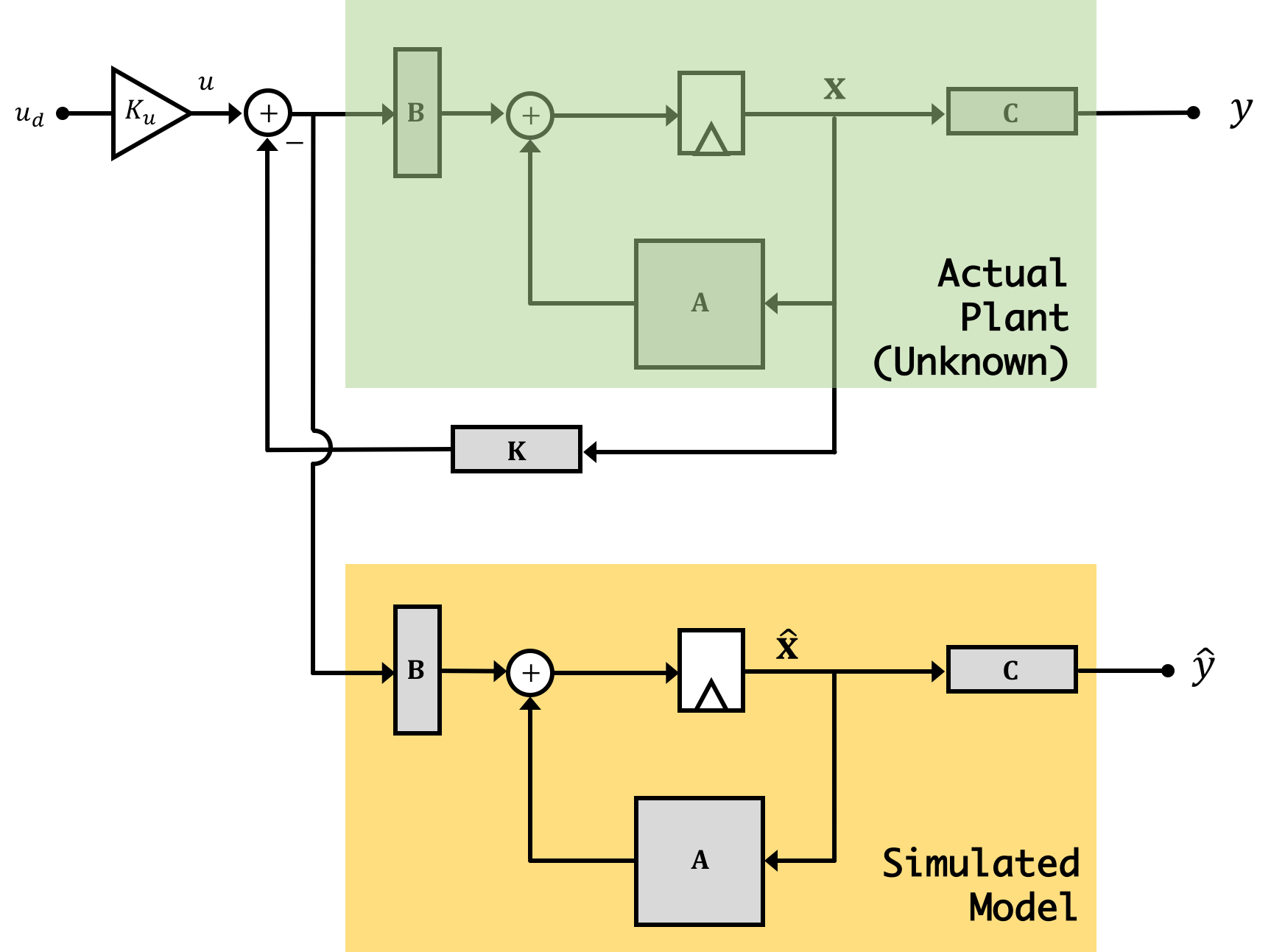
Now why are we doing this? Because the observer is a simulation, we have access to all "parts" of it, including the states. If we can make sure that our simulation accurately reflects the behavior of the real system, it probably means that the states of our simulated system are similar to what the actual states are. If this is so, we can use these simulated states to fill in for the "real" states that we cannot get access to from our real plant. We can multiply these estimated states by a gain vector \(\textbf{K}\) in just the same way as we were doing with our regular states from before. Diagramatically what we're doing is illustrated below:

Of course, our goal is to have our estimated states track really well the real-life states so ideally we'll be able to say: \(\hat{\textbf{x}}[n] \approx \textbf{x}[n]\) at which point the above would simplify back to what we really want (effective full state feedback): \[ \textbf{x}[n+1] = \textbf{A}\textbf{x}[n] - \textbf{B}\textbf{K}\textbf{x}[n] + \textbf{B}u[n] \]
But is it really that simple? Unfortunately no, and we'll go over why in teh following sections.
Now it is super important to remember/grasp/understand that there are two different "plants" in this combination of a physical and a virtual (observer) system. The physical plant exists and produces outputs that we can measure, it is the plant we are trying to control. The second plant is part of our observer and it is virtual. We are responsible for evolving the observer's state and computing its outputs, a process we often refer to as simulation in real time. Implementing an observer requires additional lines of code, and usually more computation. This is partly why 6.302.1x requires a faster microcontroller than 6.302.0x (along with model construction, which we will cover in the last week). Doing all the regular calculations to implement full-state feedback (state measurements and several multiplications and additions) are few enough that an Arduino Uno could handle it. But the additional arithmetic operations required to update the observer state on each iteration requires enough additional computation that the Arduino Uno can not keep up.
Using simulation alone to learn about observers can be confusing, because there is no difference between the physical plant and the virtual observer plant, everything is being simulated. The idea that one set of states are simulated as part of the control algorithm, and one set of states are simulated to act as a stand-in for the physical plant, is a subtlety easily missed when first learning this material. It is important to recognize that in our Python simulations, our simulation is simulating two things: The first is our real system, and the second is a simulation (our observer). When it comes time to deploy this on the levitating copter arm, the universe and Newtonian Physics will take care of "simulating" the first state space system (our physical one), and on our microcontroller we'll be left only needing to implement/simulate the observer version.
For 6.302.1x, coming up with an observer is actually really easy. Because we are already modeling our system in discrete time, this form can be directly entered into our microcontroller (the Teensy which will be actually running our observer), and therefore we really don't need to do much. You can think of the previous two weeks as looking into ways of coming up with observers, in a sense.
If you go on in your studies, or have already learned, about state space in continous time, and maybe you've already generated a continuous time model of your system, at this point what you'd need to do is discretize your model so that it would be compatible with a discrete time system like a microcontroller. We won't go into that here, but just be aware that we're getting off a bit easy in this step of generating our observer in 6.302.1x since we've already put in the work about modeling in discrete time!
We're going to set up an observer in our code now. Download the Lab03 Code File here!. It is significantly different that the previous two weeks' of code so make sure you're working in this new version!
First thing you'll notice is that an additional file is coming along with the code. You don't need to do anything with that file, but in case you're interested, that additional file, called linmath.h, is a library written by Wolfgang 'datenwolf' Draxinger that conveniently gives us access to some linear math operations for \(3\times 3\) and \(4 \times 4\) matrices (rather than clogging our code up with lots of for loops we'll just use this!)
There are a series of simulation matrices representing our \(\textbf{A}\), \(\textbf{B}\), and \(\textbf{C}\) matrices). We will use these matrices for simulating our observer, and therefore they need to be filled in with your three state model we've derived over the last two weeks. For example, if you wanted an \(\textbf{A}\) matrix that was the identiy matrix \(\textbf{I}\) (you don't btw), you'd just do:
//A matrix
mat3x3 A = {
  {1, 0.0, 0.0},
  {0,   1.000, 0.0},
  {0.0,     0, 0.0}
};
To keep the GUI from being overcrowded in Lab03 we're going to hardcode our desired feedback gains (use a set of three that you found worked well for this system in Lab 02). Those should be entered into the vec3 K matrix towards the top of the code. For flexibility you will still have access to the "Direct" and "Desire" controls in your code, however, and those will need to be set (Direct in particular) when running.
There is also an L matrix at the top. Leave this with zeros in it for the moment.
Note: the \(\textbf{B}\), \(\textbf{C}\), and \(\textbf{K}\) matrices are all written in the same "shape", when we know that they aren't. Don't worry we take care of that discrepency when we actually use the matrices in the loop.
In general, the bulk of the code remains the same. However every time through the loop, after calculating the real state values, but prior to assigning an outpu tvalue our code will update its observer . This involves performing the matrix math involved in calculating our \(\hat{\textbf{x}}[n+1]\) based on current information! This is carried out in the section of code below:
// 1. UPDATE STATE
  vec3 temp1, temp2, temp3, temp4;

  // xhat[n+1] = A*xhat[n] + B*u[n] + L*(y[n] - C*xhat[n])::
  mat3x3_mul_vec3(temp1, A, xhat); // A*xhat
  vec3_scale(temp2,B,u); // B*u
  vec3_scale(temp3, L, (y-vec3_mul_inner(C,xhat))); // L*(y-yhat) = L*(y-C*xhat)
  //vec3_add(xhat,temp2,temp1); // A*xhat+B*u
  vec3_add(temp4,temp2,temp1); // A*xhat+B*u
  vec3_add(xhat, temp4,temp3); // xhatnew = A*xhat + B*u + L*(y-yhat)
Following that is a piece of code that decides whether to control our system using the real states or the estimated states (controlled through a GUI-based slider). After this, the code is very similar to Labs 1 and 2, with a few additional details that aren't important for our learning here.
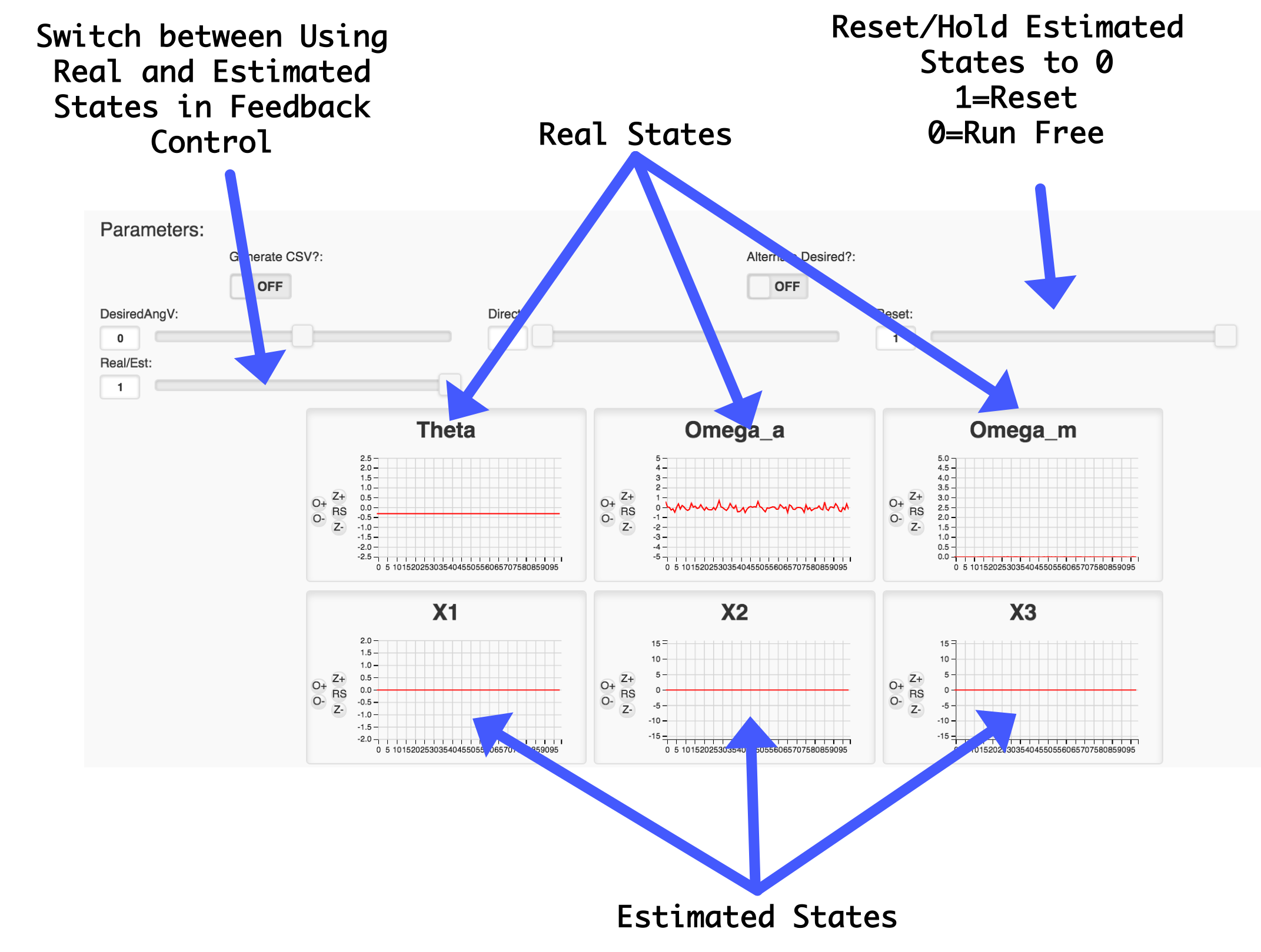
Lab 03's GUI has six plots in it. They come from the following pieces of data being sent up:
packStatus(buf, rad2deg*angleV, rad2deg*omegaArm, motor_bemf, rad2deg*xhat[0], rad2deg*xhat[1], xhat[2], float(headroom));These values are:
rad2deg*angleV: Arm angle in degreesrad2deg*omegaArm: Arm angular velocity in degrees per secondmotor_bemf: Motor Back EMF (in Volts)rad2deg*xhat[0]: Estimated state one (\(\hat{x}_1\)) (in degrees)rad2deg*xhat[1]: Estimated state two (\(\hat{x}_2\)) in degrees per secondxhat[2]: Estimated state three (\(\hat{x}_2\)) (in Volts)For the pursposes of learning, we'd like to be able to switch back and forth between using the real states and the estimated states to compare and contrast their capabilities. There is a "Reset Slider" near the top whose job is to "zero" the estimated states since they can sometimes drift to crazy amounts when run open loop (what we're doing this first time). Use this to re-zero your esimated state so you can see how quickly they diverge from the real states (which are also plotted!)
We've also included a slider that will allow you to during operation switch between using the actual states and the estimated states. It is set up such that when set to 0, the real states are used. When set to 1, the estimated states are used.
For quick review the GUI's functionality for Lab 03 is depicted below:
Fill in the matrices and add in gains that you've found working for your system (don't forget to also hardcode the Ku gain with your precompensator gain value \(K_u\)! Once completed, upload the code and start the GUI. Note that once power is turned on your system will start running (unlike in previous labs) since we have hardcoded non-zero gains for the gain vector!
With your system turned on, zero out the states and keep them zeroed. Bring the directV term up in value until the system is running horizontally like before (the value you use for this should be similar to what you needed in the last lab.
If we were to then unzero our estimated states, our system will look like the following:
The observer when run in parallel with this is not necessarily affected by the feedback so its own natural frequencies will just be its originals, or those of the \(\textbf{A}\) matrix. This is an important thing to realize! The observer as set up like this is potentially not stable! So if you run it, we can't necessarily expect it estimated states to not diverge!
With the system running stably, unzero the estimated states and observe what they do. Which ones track somewhat well with what is happening with the real states? Which ones don't? Why do you think that is?
If the estimated states deviate a significant amount from their actual siblings, re-zero them and then with them again running freely, consider switching to estimated-state control. How well does the system work? Does the system work at all?
Aside from the fact that the observer is potentially not stable, if we were to potentially be able to start our observer in the same initial state as our real plant and then give our observer the exact same inputs as our real system (inputs which by the way keep the real plant stable), couldn't we expect the output of the observer to effectively mimic the output of the real plant? Generally no. To figure out why our estimated states are not tracking very well, let's consider the following simple two-state double integrator system where the input is acceleration \(a\) and the output is height \(h\).
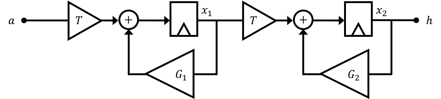
We'll say our two states are \(x_1\) and \(x_2\) so that:
\[ \textbf{x} = \begin{bmatrix}x_1\\x_2\end{bmatrix} \]We can come up with an "error" vector \(\textbf{e}\) such that:
\[ \textbf{e}[n] = \textbf{x}[n] - \hat{\textbf{x}}[n] \] and we'll call the terms within that vector: \[ \textbf{e} = \begin{bmatrix}e_{1}\\e_{2}\end{bmatrix} \]At the beginning, the real and simulated system's start at rest (all states are 0). We're going to provide a unit step input to the system. Assume that in our plant and in our observer that we built, both \(G_1\) and \(G_2\) are \(1\) and that our timestep \(T=1\). After 10 seconds (10 time steps) what will the values of our error vector be?
What now would happen if we still run our observer with gains of \(G_1=G_2=1\), but in reality, life gets in the way and changes the actual value of \(G_1\) to be \(0.95\), a relatively small \(5%\) error from what we assume. If we give both our plant and our observer a unit step input, at 10 seconds (when \(n=10\)) what will the values of our error vector be? Answer to three significant figures. Read the solution afterwards!
If you've been paying attention to how things have been going, our model is not perfect...We basically ignore gravity, linearize like crazy when it comes to thrust, assume the motor doesn't have an inductor, and lots of other things. Basically our model, while decent and grounded in some physics, is probably not going to be able track our real-life system open loop. Some parts of it might, but these are generally parts that are directly connected/influenced by the input. The further removed a state is from the input, the more likely that errors can come into play! You should have seen evidence of that in your system when you ran it! Our system has lots of discrete time integration/accumulation in it and over time slight deviations in the model compared to actual system performance will cause serious deviation of our estimation of states!
Now just like we use feedback to compensate for the fact that our system is not perfect we can use feedback to do the same thing for our observer! That's right, the solution is to place the observer itself into feedback! But how? Like shown in the image below:
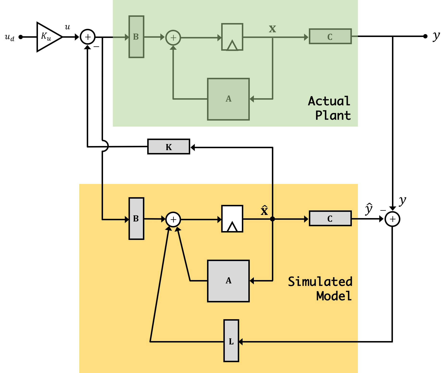
We're now going to create an output error signal we'll call \(e_y[n]\) which we'll define as: \[ e_y[n] = y[n] - \hat{y}[n] \] We'll use this error signal, multiplied by a gain vector \(\textbf{L}\) to correct the system's states.
Note we're using feedback towards a distinctly different way in the observer when compared with how we used it for the greater system. In the first two labs (and really in all the labs in 6.302.1x) we're using state feedback to get our output to be what we want. In the case of the observer, we're using output feedback to get our estimated states to be what we want (namely as close to possible as the actual state values). This is as much a feedback problem as when we're controlling the system's output, and we'll want our observer to be able to converge quickly on the actual values so that we can use them in a timely manner to control the greater system. In fact, we'll want the eigenvalues/natural frequencies of the system to be at least \(2\times\) and ideally more faster than the eigenvalues/natural frequencies of our fedback system. This is critical since if our observer takes too long to arrive at what the states are (on the same order of time dynamics as the actual plant's state variables themselves), by the time we have good information, it'll be too late to use it!
To analyze the observer's ability to converge on the correct state we need to return to our error vector \(\textbf{e}\) that we discussed on a previous page: \[ \textbf{e[n]} = \textbf{x}[n] - \hat{\textbf{x}}[n] \] Deriving state space expressions for the observer results in: \[ \hat{\textbf{x}}[n+1] = \textbf{A}\hat{\textbf{x}}[n] - \textbf{BK}\hat{\textbf{x}}[n] + \textbf{B}u[n] + \textbf{L}\left(y[n] - \hat{y}[n]\right) \] And then our actual plant state space expression would be: \[ \textbf{x}[n+1] = \textbf{A}\textbf{x}[n] - \textbf{BK}\hat{\textbf{x}}[n] + \textbf{B}u[n] \] Subtracting the expression for the estimated state\(\hat{\textbf{x}}\) from that of the actual state\(\textbf{x}\) we can come up with a state space expression for the error vector: \[ \textbf{e}[n+1] = \textbf{A}\textbf{e}[n] -\textbf{L}\left(y[n] - \hat{y}[n]\right) \] and if we remember that: \[ y[n] - \hat{y}[n] = \textbf{C}\left(\textbf{x}[n] - \hat{\textbf{x}}[n]\right) \] ...we can then factor some stuff out so that it will be: \[ \textbf{e}[n+1] = \textbf{A}\textbf{e}[n] -\textbf{LC}\left(\textbf{x}[n] - \hat{\textbf{x}}[n]\right) \] or finally: \[ \textbf{e}[n+1] = \left(\textbf{A}-\textbf{LC}\right)\textbf{e}[n] \]
Now using the what we've learned about feedback and control in Week 1 and 2, this equation format should look very familiar. When placed into feedback like this using the difference of the two outputs (estimated and actual) as well as a feedback observer gain of \(\textbf{L}\) we can adjust the eigenvalues (natural frequencies) of the error signal, which means we can control how quickly our observer can correct its estimated state vector to match with the actual state vector!
If we think of the error vector and our original state vector as now as components of a much larger state space system (with state vector shape of \(2\times m\) where \(m\) is the number of states) like that shown below and interesting characteristic will appear: \[ \begin{bmatrix}\textbf{x}[n+1] \\ \textbf{e}[n+1]\end{bmatrix} = \begin{bmatrix}\textbf{A} - \textbf{BK} & \textbf{BK}\\0 & \textbf{A}-\textbf{LC}\\ \end{bmatrix}\begin{bmatrix}\textbf{x}[n] \\ \textbf{e}[n]\end{bmatrix} \] The new \(2m \times 2m\) \(\textbf{A}\) matrix takes on the shape of a Block Upper Triangular Matrix which can be shown to have the following property: \[ \det\begin{pmatrix}M_{11} & M_{12} \\ 0 & M_{22}\\ \end{pmatrix}= \det(M_{11})\operatorname{det}(M_{22}) \] This independence of the determinant, ultimately means that the eigenvalues of the entire system will be just the eigenvalues from our \(\textbf{A}-\textbf{BK}\) expression and the eigenvalues of our \(\textbf{A} - \textbf{LC}\) expression! What this is saying is that the we can pick the values of our feedback gains \(\textbf{K}\) and our observer feedback gains \(\textbf{L}\) independently so we don't have to interweave their derivation. If we can pick an \(\textbf{L}\) to get our estimated states to converge quickly enough, then we can use the same tools we used in Week 2 to derive our gain \(\textbf{K}\)! So long as we can get the state error \(\textbf{e}\) to converge much faster than the state dynamics themselves we'll be good to go!
Finally instead of having a hybrid state space expression with the error vector, we can instead have one comprised of our \(m\) real states and our \(m\) estimated states like so: \[ \begin{bmatrix}\textbf{x}[n+1] \\ \hat{\textbf{x}}[n+1]\end{bmatrix} = \begin{bmatrix}\textbf{A} & -\textbf{BK}\\\textbf{LC} & \textbf{A}-\textbf{LC} - \textbf{BK}\\ \end{bmatrix}\begin{bmatrix}\textbf{x}[n] \\ \hat{\textbf{x}}[n]\end{bmatrix} + \begin{bmatrix}\textbf{B}\\\textbf{B}\end{bmatrix}K_u u_d[n] \] and \[ y[n] = \begin{bmatrix}\textbf{C}, 0...0\end{bmatrix}\begin{bmatrix}\textbf{x}[n] \\ \hat{\textbf{x}}[n]\end{bmatrix} \]
acker to arbitrarily place our natural frequencies was that our system was what we call "controllable". What this basically means is that the system can have its natural frequencies changed however we want. There's a way to check for controllability using matrix rank and some other stuff, but for now we'll assume that our system's are all controllable.
Interestingly, there's a complementary criterion to that known as "observability" which means that we can arbitrarily move the natural frequencies of a system observer around, and while we'll avoid the derivation here, we can also assume our system's have this property. Therefore, just like we had complete theoretical freedom in moving the eigenvalues (natural frequencies) of our plant around by manipulating \(\textbf{K}\) in the expression \(\textbf{A}-\textbf{BK}\) we have will have the same sort of freedom in picking our \(\textbf{L}\) vector in the \(\textbf{A} - \textbf{LC}\) expression. Because of the shapes of our matrices however we need to make some changes if we'd still like to use the Ackermann method, with us instead using the transpose of the \(\textbf{A}\) and \(\textbf{C}\) matrices (so they have the same shape as the \(\textbf{A}\) and \(\textbf{B}\) matrices from week 02 when we used this for system eigenvalue placement/gain determination). We will also need to transpose the result coming back since \(\textbf{L}\) is \(1\times m\) (same dimensions as \(\textbf{C}\) and not \(m \times 1\) like the \(\textbf{K}\) matrix. In numpy you can quickly transpose a matrix via the .T method like so:
obs_nat_freqs = [0.95,0.95,0.95]
L = acker(A.T,C.T, obs_nat_freqs).T
print("L values:")
print(L)
Go ahead and add these several lines of code to an appropriate location in your Python code from Week 02 in order to generate values for your \(\textbf{L}\) vector based on your model. Just to reiterate, note that in picking these values, we are not using the \(\textbf{K}\) values in any way!
If we remember from picking gains for system control in Week 02, we were mathematically unrestricted in what we asked for, but realistically restricted because of model/system limitations. Will the same situation arise here? Since an observer is all a simulation, will it matter if we pick a really small set of desired natural frequencies? Yes and No: We don't have to worry about state values being too high or our command signal being too large, but we do need to worry about too much \(\textbf{L}\) uneccessarily amplifying output noise. Because small natural frequencies/eigenvalues are generally associated with larger \(\textbf{L}\) values, this means that very fast responding observers will potentially cause trouble.
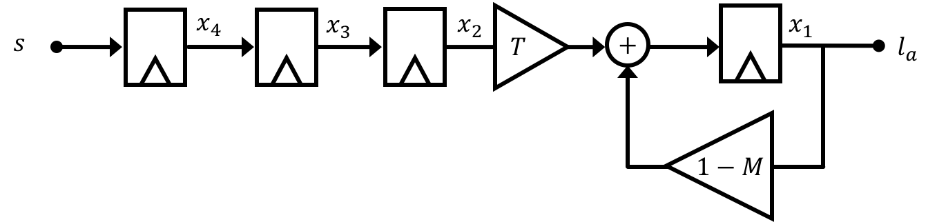
The rationale for this is the following: In looking at our estimator the \(\textbf{L}\) is applied to the \[ \hat{\textbf{x}}[n+1] = \textbf{A}\hat{\textbf{x}}[n] + \textbf{B}u[n] + \textbf{L}\left(y[n] - \hat{y}[n]\right) \] If we were to add in an additional signal \(s[n]\) representing a small amount of noise on the output, it would go where the output value \(y[n]\) is located (think of it as a noise signal "on top" of the output signal. \[ \hat{\textbf{x}}[n+1] = \textbf{A}\hat{\textbf{x}}[n] + \textbf{B}u[n] + \textbf{L}\left(y[n] + s[n] - \hat{y}[n]\right) \] We can consequently adjust our error vector's \(\textbf{e}\) state space expression: \[ \textbf{e}[n+1] = \textbf{A}e[n] - \textbf{L}\left(y[n] - \hat{y}[n] + s[n]\right) \] and then: \[ \textbf{e}[n+1] = \left(\textbf{A} - \textbf{LC}\right)e[n] - \textbf{L}s[n] \] If we try to get really small eigenvalues for the observer, this generally comes about from having really large values inside \(\textbf{L}\). The problem with this can become apparent in a steady state situation where we say that \(n \approx n+1 \approx n_{\infty}\) and so \(\textbf{e}[n_{\infty}] = \textbf{e}_{ss}\) and \(s[n] \to s_{o}\). In that situation: \[ \textbf{e}_{ss} = \left(\textbf{A} - \textbf{LC}\right)\textbf{e}_{ss} - \textbf{L}s_{o} \] and therefore: \[ \textbf{e}_{ss} = \left(\textbf{I}-\left(\textbf{A} - \textbf{LC}\right)\right)^{-1}\textbf{L}s_o \] Now if we're picking \(\textbf{L}\) to make really small eigenvalues we'd therefore expect that the magnitude of the eigenvalues for \(\textbf{A} - \textbf{LC}\) will be about 0 or: \[ \left|\lambda_i\left(\textbf{A} - \textbf{LC}\right)\right| \longrightarrow 0 \] The spectral mapping theorem can be used to show that if a matrix \(\textbf{G}\) is based on some function call on another matrix \(\textbf{H}\), \(f(\textbf{H})\), then the eigenvalues of \(\textbf{G}\), which we'll denote as \(\lambda_i\left(\textbf{G}\right)\) can be shown to be \(f(\lambda_i\left(\textbf{H}\right)\). Applying that here, if the eigenvalues of \(\lambda_i\left(\textbf{A} - \textbf{LC}\right)\) are small, then the following are approximately 1: \[ \lambda_i\left(\left(\textbf{I}-\left(\textbf{A} - \textbf{LC}\right)\right)^{-1} \right) \approx 1 \] So if the eigenvalues are small that front term ends up just having a lot of eigenvalues approximately equal to 1, that basically means our error terms will end up being aout \[ \textbf{e}_{ss} \approx \left(1\right)\textbf{L}s_o \] and since we know that \(\textbf{L}\) is large this means our error will be large.
Now in the first half of this lab where we ran our observer, we saw that our observer's estimated states quickly deviated from the actual states while running in feedback. In the previous two sections we just figured out how to use output feedback to make our observer track the actual states. We're going to do that now on our microcontroller!
Using your Week 2 python code, select a set of observer gains to place the observer's natural frequencies at [0.95, 0.95, 0.95]. Enter these three \(\textbf{L}\) values into the L matrix located at the top of the microcontroller code. Upload and like before start up your system.
[0.90, 0.90, 0.90]. What about [0.8, 0.8, 0.8]? What about [0.5, 0.5, 0.5]?
An intermediate between a full observer and full-state feedback is when we have access to some of a system's state variables but not all. We can then come up with an observer that uses only partially what it has. In general the more "real" information you can get the better, but there are definite exceptions to this. For example in the case of our observer, the estimated state \(\hat{x}_2\) which corresponds to the arm angular velocity signal \(\omega_a[n]\) is significantly less noisy than the real life signal! At least on my setup anyways. Part of this comes from teh fact that our "real" measurement of angular velocity isn't actuall real. It is based on taking a discrete time derivative of multiple angle measurements over time, and this can be noisy. But also there is a lot of vibration in our system so this is noisy as well. Without access to something such as a gyroscope this may be a better bet....in fact one thing you may have noticed when switching between actual and estimated state control is that the system seemed less noisy/gross-sounding using the estimated states! This should make sense based on this discussion!
To come up with a hybrid modify the command signal lines in the code:
    if (real_est == 1){ //if using estimated (real_est==1):
    u = Ku*desiredV - K[0]*xhat[0] - K[1]*xhat[1] - K[2]*xhat[2] + directV;
  }else{ //if using actual states (real_est==0)
    u = Ku*desiredV - K[0]*angleV - K[1]*omegaArm - K[2]*motor_bemf + directV;
  }
to use a mix of actual and estimated states. It may make sense to use the actual angle, for example, but to avoid using the actual state in the case of angular velocity or back EMF for reasons of noise or built-in offset as discussed above!
Replace the estimated angular velocity state with the actual one! should seem less noisy in its response, however its ability to respond to disturbances will be more limited. For example, check to see how well your system responds to a tap. Your system will respond more sluggishly to correct that in the case of an observer.
Do you notice any downsides to the system response with the observer? Does it seem more sluggish? Less stable?
So in the end even in the case where you do have access to the true states it can sometimes be advantageous to instead use estimates of those states for the purposes of noise suppression and keeping things compatible with our model. It seems like cheating, but it isn't! It is very cool!
Now that we've (hopefully) succssefully got an observer working in real life, what/how we use it will hopefully make a bit more sense. Now we'll spend a bit of time simulating the effect of an observer in other systems.
Reconsider our anesthesia system from Week 2:
We said at the beginning of Week 3's notes that this may be an example of a system where it might just not be possible to measure all the states and use them in full state feedback. Instead we're going to come up with an observer and use that.