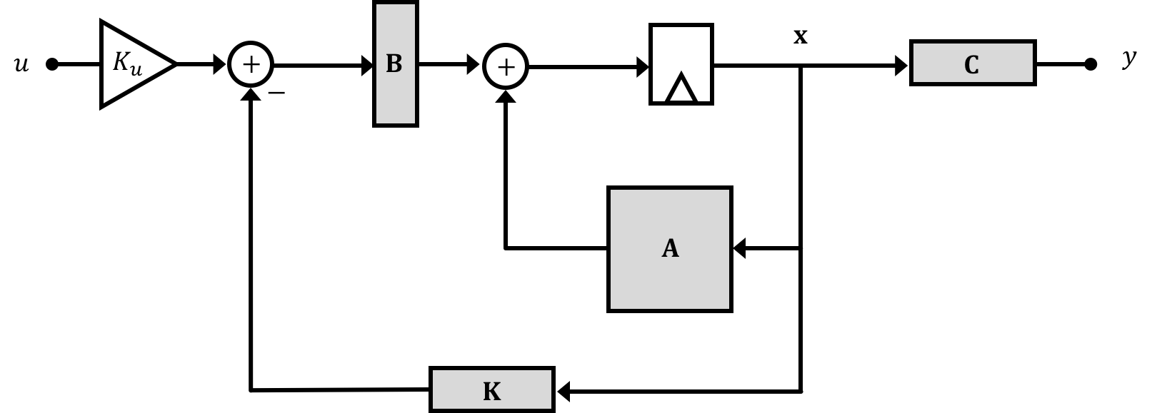
Based on what we discussed in the notes, while our propeller arm system has a plant expressed with the matrices derived on the previous page (of which the eigenvalues of the \(\textbf{A}\) matrix are its natural frequencies) , we can use state feedback in order to modify those eigenvalues towards the goal of stabilizing the system:
For Week 1, we're just going to roughly gauge numbers to pick based on experience in 6.302.0x. In Week 2, we'll look at more quantitative ways of assigning the feedback gains.
Starting with \[ \textbf{K} = \begin{bmatrix}K_1\\K_2\\K_3\end{bmatrix}=\begin{bmatrix}0\\0\\0\end{bmatrix} \] If we wanted to implement proportional only control on the arm angle, what term would we adjust and how would we do it?
\(K_1\) is directly multiplied by the \(\theta_a\) state, and because we subtract the result of \(\textbf{K}\cdot\textbf{x}[n-1]\) we'd want a positive value fo \(K_1\) to implement proportional control. This will only make sense, however, if \(K_u\) is adjusted appropriately!
When carrying out Proportional + Derivative Control (a PD controller), a gain \(K_d\) is applied to the derivative of the error signal. In the case of state feedback to control the arm angle in our propeller setup, what value of the \(\textbf{K}\) matrix would need to be changed (and how) in order to implement derivative control?
Starting with \[ \textbf{K} = \begin{bmatrix}K_1\\K_2\\K_3\end{bmatrix}=\begin{bmatrix}0\\0\\0\end{bmatrix} \] If we wanted to implement proportional+Derivative control on the arm angle, what term would we adjust and how would we do it?
Explanation
\(K_2\) is directly multiplied by the \(\omega_a\) state, and because we subtract the result of \(\textbf{K}\cdot\textbf{x}[n-1]\) we'd want a positive value fo \(K_2\) to implement proportional control.
When carrying out Proportional + Derivative Control (a PD controller), a gain \(K_d\) is applied to the derivative of the error signal. Assuming our input stays constant, and building upon your answer above, would we need to modify \(K_u\) in order to properly implement true discrete time derivative control in our system (in conjunction with the change you stated in the situation above?)
Explanation
To quickly do a continuous time analysis we can say our error is: \[e(t) = \theta_d(t) - \theta_a(t)\] if our input (desired angle) stays relatively constant with time, then when we take the time derivative of our error we'd get: \[\frac{de(t)}{dt} \approx \frac{\theta_a(t)}{dt} \] Since one of our states is \[ \omega_a = \frac{\theta_a(t)}{dt} \] that means applying a gain onto the the system's angular velocity (gain \(K_2\)) will be the same! No modification of \(K_u\) is necessary in order to make sure derivative control is implemented!
When carrying out Proportional Control (a P controller), a gain \(K_p\) is applied to the error signal. Assuming our input stays constant, and building upon your answer above, would we need to modify \(K_u\) in order to properly implement proportional control in our system (in conjunction with the change you stated in the situation above?)
Explanation
Yes in Proportional control we drive our plant with \(K_p\) times an error signal. In the situation of our system, our error is defined as: \[ e[n] = \theta_a[n] - u[n] \] For us to implement true proportional control we need to drive our plant with: \[ K_pe[n] \] For that to be true, the signal going into our plant must be: \[ input_[n] = K_p\left(\theta_a[n] - u[n]\right) \] As discussed above, a positive \(K_1\) will take care of part of the proportional gain implementation, but it will not take care of the \(K_p\theta_a[n]\) term, so we need to also have \(K_u = K_p\) in order to implement proportional control fully.
If you'd like, using sympy or another symbolic matrix library, calculate \(K_u\) out officially using our expression for it below:
\[
K_u = \left(\textbf{C}\left(\textbf{I}-\textbf{A}+\textbf{BK}\right)^{-1}\textbf{B}\right)^{-1}
\]
If you coded up/implemented all of your matrices properly, you should get the same value for \(K_u\) as we reasoned through in the question above (see solutions on this page!). We can discuss this more in the forum as needed! This is a good sanity check that you are implementing your state space model appropriately in code if you're doing that!
Can we design a better position controller using state feedback with all the states, not just the arm angle? For this experiment you are going to try, but you will find that we really do not have the tools to find the best values for the \(K_i's\), but perhaps you can find pretty good ones. And in addition, you will encounter a problem with scaling variables, an important practical matter.
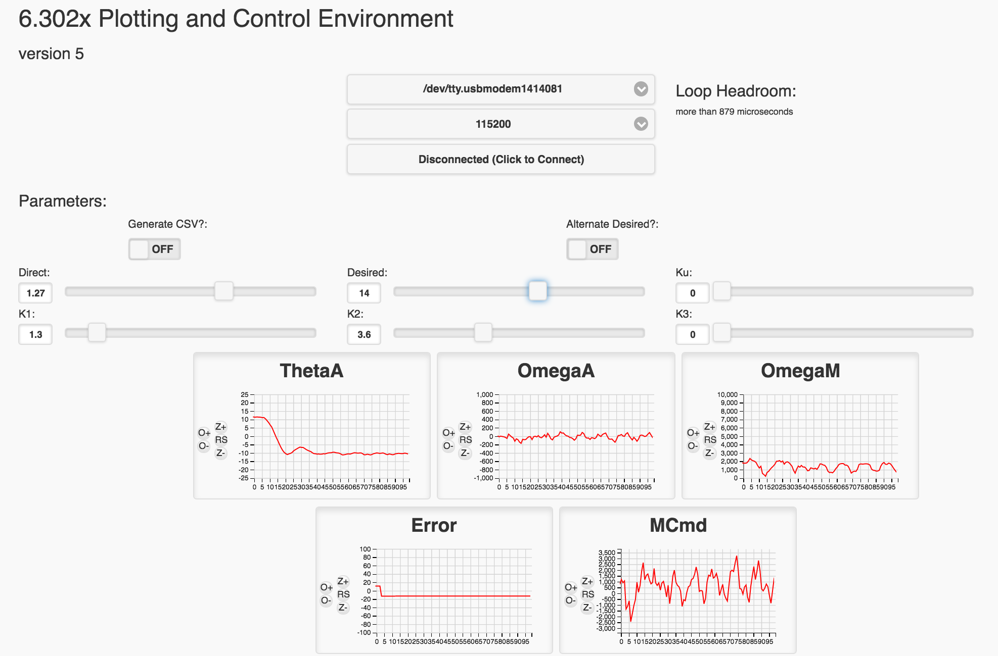
Recall that running your code GUI will look like the following:
Your task is to find the line of code that does this:
   // calculate the motor command signal here:
  float motorCmd = directV;
and modify it to implement state feedback on all three states. Inside the code the three \(\textbf{K}\) gain matrix parameters are specified as variables K1, K2, and K3 (tied to sliders)
The variable directV can be thought of as an offset which we'll use to cancel gravity out, as well as sort of compensate for other linearizations that we undertook. It is tied to a GUI slider.
Many of our system parameters are also prsent:
angleV is arm angle \(\theta_a\)angleVderv is arm angular velocity\(\omega_a\)motor_omega is motor velocity \(\omega_m\)motor_bemf is the motor's back EMF \(v_{emf}\)Ku is the precompensator gain (tied to GUI slider)desiredV is the input signal \(u\) (tied to slider in the GUI)You will be using these variables to implement measured-state feedback on the states we will discussing in what follows. When you make changes to the Teensy code, upload it to your Teensy and then start the GUI. And whenever running an experiment, start by setting all the sliders to zero, and then adjusting the direct value so that the propeller spins fast enough to lift the arm to a little below the horizontal. Then adjust the various gains for the controller you are trying to implement. <\p>
Once you have a stable operating system from adjusting the direct offset term as well as \(K_1\) and \(K_2\) and \(K_u\), add in some gain on the \(K_3\) term. You should notice the system completely stop running even for extremely low values (\(K_3 = 0.1\)). In fact you should see it start to obtain a periodic burst activity Why is this?
While both \(\theta_a\) and \(omega_a\) remain relatively small in value during normal operation (check your plots!), the motor speed (measured in radians per second) is rather large numerically (again check your plot). Consequently when we apply even a small amount of gain to the motor speed state, (relative to what we're doing with \(K_1\) and \(K_2\) the resulting signal is very negative. This isn't saying we can't utilize the \(\omega_m\) state for feedback, rather the gain we apply to it must be even smaller than what we're thinking. We must think of another way to represent that state.
One way to fix this scaling issue is to replace our motor speed state variable \(\omega_m\) with the back EMF voltage (\(K_e\omega_m = v_{emf}\). This has two advantages:
When combined, these two features mean this signal could be a more readable state, and when we really pursue proper full-state feedback in Lab 2 this will be the state we use, however we will come back to the implications of differences in signal/state units during that discussion.
In order to work with this new state, we need to modify our state space model a bit by replacing and adjusting the third row (corresponding to the motor velocity state) as well as any states which it modifies. This will result in changes to matrix of the state vector as well as \(\textbf{A}\) matrix value \(a_{23}\) to "undo" the new \(K_e\) implied in the state as well as the the \(b_{31}\) term of \(\textbf{B}\) matrix: \[ \begin{bmatrix} \theta_a[n] \\ \omega_a[n]\\ K_e\omega_m[n]\\ \end{bmatrix} = \begin{bmatrix} 1 & T & 0\\ 0 & 1 & \frac{TK_tL_a}{K_eJ_a}\\ 0 & 0 &\left(1-\frac{TK_mK_e}{J_m\left(R_m+R_s\right)}-TK_f\right)\\ \end{bmatrix} \begin{bmatrix} \theta_a[n-1] \\ \omega_a[n-1]\\ K_e\omega_m[n-1]\\ \end{bmatrix} + \begin{bmatrix} 0\\ 0 \\ \frac{TK_eK_m}{J_m\left(R_m+R_s\right)} \\ \end{bmatrix}v_{pwm}[n-1] \] and also the following, although since we don't use that third state in our output it doesn't change from before much. \[ y = \begin{bmatrix}1 & 0 & 0\\ \end{bmatrix} \begin{bmatrix} \theta_a[n] \\ \omega_a[n]\\ K_e\omega_m[n]\\ \end{bmatrix} \]
Change the motor speed state you're currently using to apply a gain in the to the back emf instead. To modify your code replace the line at the top of the code that says String config_message_lab_1_6302d1 = with the following (this adjusts the plots to expect/label for Back EMF and not Omega
String config_message_lab_1_6302d1 = "&A~Desired~5&C&S~Direct~O~0~2~0.01&S~Desired~A~-90~90~1&S~Ku~U~0~10~0.01&S~K1~B~0~10~0.01&S~K2~C~-0~10~0.01&S~K3~D~-0~10~0.01&T~ThetaA~F4~-100~100&T~OmegaA~F4~-1000~1000&T~Vemf~F4~0~5&T~Error~F4~-100~100&T~MCmd~F4~0~5&D~100&H~4&";And change the line:
packStatus(buf, angleV*rad2deg, angleVderv*rad2deg, motor_omega, errorV*rad2deg, motorCmdLim, float(headroom));So that it says the following (reporting motor back EMF rather than motor velocity \(\omega_m\)):
packStatus(buf, angleV*rad2deg, angleVderv*rad2deg, motor_bemf, errorV*rad2deg, motorCmdLim, float(headroom));
Reload the code onto the microcontroller, restart the server (press control C if you don't know how), and then restart. Addition of a bit of gain on the third state now, while not necessarily giving a much improved response, is at least not completely removing the command signal now!
In Week 1, we looked into the idea of full state feedback where we could use information about a system's states in conjunction with assigned gains on each state to implement feedback control and modify a system's response. From the perspective of the state space approach, this feedback was changing the natural frequencies/eigenvalues of the system's \(\textbf{A}\) matrix by replacing it with a modified \(\textbf{M}\) matrix where \[ \textbf{M} = \textbf{A} - \textbf{B}\textbf{K} \] This methodology is very powerful and generally more extensible than the simple one-line difference equations that we go over in 6.302.0x. For example, it is relatively easy to add an additional state to an existing state-space model, but doing the equivalent in a purely difference equation form can prove to be difficult.
While this idea of state feedback is great, the question remains how do we go about picking the values that make up the \(\textbf{K}\) matrix? Remember our \(\textbf{K}\) matrix gets multiplied with our state vector \(\textbf{x}\) to provide a feedback scalar term: \[ \textbf{K} \textbf{x}[n] = \begin{bmatrix}K_1, K_2,\ldots,K_m\end{bmatrix} \cdot \begin{bmatrix}x_1[n]\\x_2[n]\\\vdots\\x_m[n]\end{bmatrix} = \sum_{i=1}^m K_i x_i[n]. \]
We'll start to look at ways of going about doing this by first picking where we want our natural frequencies to be, and then solving for the appropriate gains that will achieve this for us. We'll see that for low-order systems, this isn't too hard of a task to do, (though even for a \(2\times 2\) case it gets tedious), but for larger systems it becomes more and more difficult and we really end up needing numerical techniques. These numerical techniques, however are not just plug-and-play...they'll give you values for your \(\textbf{K}\) but it doesn't mean they're good to just plug into a real system! We'll look into how to use some of these techniques for design and go from there.
Finally we'll look at Linear Quadratic Regulators (LQR), some of the math behind them, and how to work with them. LQR gives us a bit more control over what values we let the states and inputs go to during operation, but this additional freedom can be hard to use.
One of the benefits of state space, is that it is a very computationally friendly approach to modeling and controlling systems. Rather than focus just on the math, we also want to get some experience using some modern tools that are helpful when dealing with state space systems (particularly as you go to larger numbers of states).
A lot of controls tutorial will utilize MATLAB in their examples, and if you have access to tha software, it is definitely worth your time to learn some of its capabilities. It is really, really powerful (not just in controls) and one of the standards in many fields of engineering. It is an expensive piece of software for a single learner or individual to acquire, however, and so to avoid requiring students to buy a license, we'll be using Python in this course!
If you've been running the lab experiments for 6.302.0x and/or 6.302.1x we've already tricked you into putting Python on your machine. There are a number of very nice free Python packages that we're now going to download (which many of you may already have) in order to start doing some modeling as well as calculation of system gains!
pip for Python really makes installing general standard libraries pretty easy. To get the libraries listed above, go into a command shell/Power Shell, or Terminal and type the following:
pip install library_name
Where you'll replace library_name with the name of the library we want. Note, depending on your OS, you may need to do pip3 in place of pip.
We'll want the following libraries so install each of them. These *should* be easy to get going, and some of you may already have them installed, depending on your system!
numpyscipymatplotlib...this one will take a bit...go eat some cookies while it installscontrol A fantastic Python-based controls library that is very similar in style and functionality to MATLAB. It was written and maintained by Astrom and Murray out of Caltech to support their very nice text book. Documentation Here Let's start with an example:
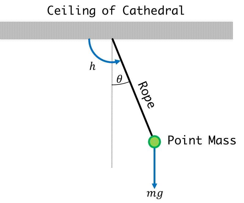
You were in a cathedral having some sort of crisis of faith or something and noticed a point mass suspended on the ceiling. Every so often wind could blow in through one of windows, generate a torque, and cause it to move. Instead of "wondering what it all means", you instead find solace in creating a state space model of the pendulum's motion. You come up with the following:
\[
\begin{bmatrix}\theta[n] \\ \omega[n]\end{bmatrix} = \begin{bmatrix}1 & T\\-\frac{gT}{l} & 1\end{bmatrix}\begin{bmatrix}\theta[n-1] \\ \omega[n-1]\end{bmatrix} + \begin{bmatrix}0 \\ \frac{T}{J} \end{bmatrix}h[n-1]
\]
where \(\theta\) is the angle of the pendulum, \(\omega\) is the angular velocity, \(\alpha\) is the angular acceleration, \(J\) is the moment of inertia which in the case of our point mass is \(ml^2\), \(h\) is an applied torque, \(l\) is the distance of the point mass from the pivot point, and \(m\) is the mass of the point mass, and \(T\) is our timestep.
Here is a more contextual explanation of some of the variables : Omega is our angular velocity, a measure of how fast we are spinning around a point. Command is the net torque on the pendulum. If it is set to zero then that means that there is no external force being applied to the system.
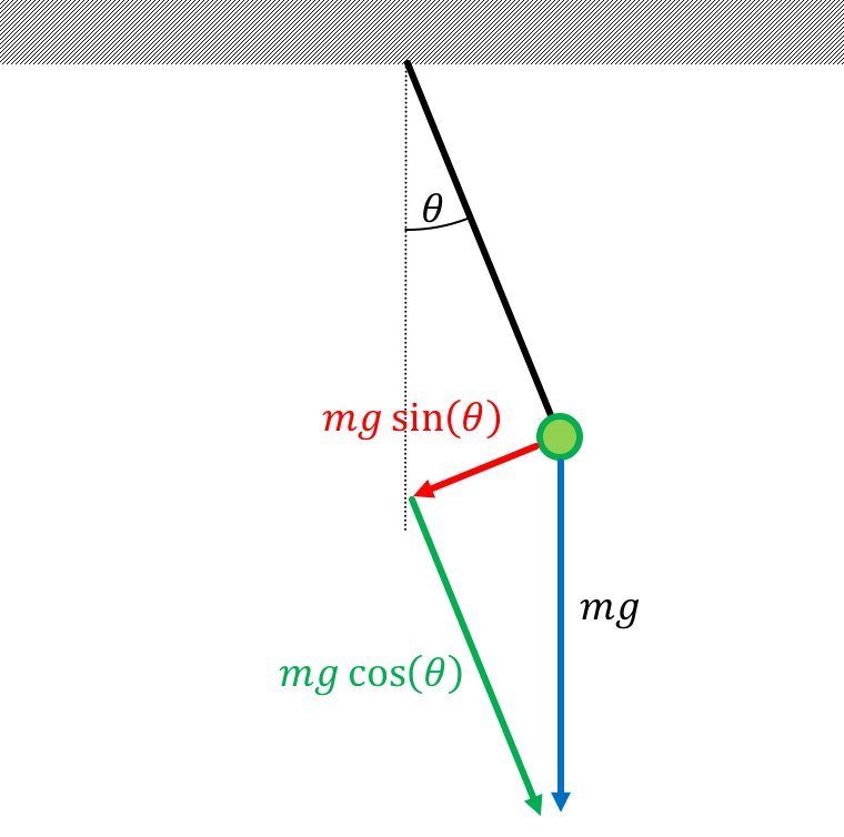
Netwon's Second Law for a Pendulum, using the terms above is (torque = angular acceleration times moment): \[ h[n] - mgl\sin\left(\theta[n]\right) = \alpha[n] J \]
The matrix equation above covers one part of our State Space System...in particular we've now got the following covered.: \[ \textbf{x}[n] = \textbf{A}\textbf{x}[n-1] + \textbf{B}u[n-1] \] But what should the other SS equation, \[ y[n] = \textbf{C}\textbf{x}[n] + \textbf{D}u[n], \] be if we want our output to be the angle?
Enter the \(\textbf{C}\), \(\textbf{D}\) matrices below for the state space representation above and \(u = h[n]\) and \(y\) being the angle?
Our state is is \(\begin{bmatrix}\theta[n] & \omega[n]\end{bmatrix}^T\). Since we want our output to only be the angle, \(\textbf{C}=\begin{bmatrix}1 & 0\end{bmatrix}\). Because our input is a torque and our output is the angle, there is no direct relationship between these two terms and therefore \(\textbf{D} = \begin{bmatrix}0\end{bmatrix} = \begin{bmatrix}0\end{bmatrix}\)
As discussed last week, when analyzing our state space model, the natural frequencies of the system are its eigenvalues, \(\lambda\), which can be determined by finding the eigenvalues of the \(\textbf{A}\), by solving for \(\lambda\) such that \[ \textbf{A} -\textbf{I}\lambda \] is singular, or equivalently, that the determinant of \( \textbf{A} - \textbf{I}\lambda \) is zero.
Eigenvalues are generally annoying to calculate but for \(2 \times 2\) matrices they are found using determinants and are therefore fun and emotionally satisfying to do.
Given the following system parameters for our pendulum above:
What are the two natural frequencies for the undamped(original) system?
Starting with: \[ \det\left(\begin{bmatrix}1 & T\\\frac{-gT}{l} & 1\end{bmatrix} - \begin{bmatrix}\lambda & 0\\ 0 & \lambda\\ \end{bmatrix}\right) = \det\left(\begin{bmatrix}1-\lambda & T\\\frac{-gT}{l} & 1-\lambda\end{bmatrix}\right) = 0 \] We'll end up with an expression: \[ \left(1-\lambda\right)^2 + \frac{T^2g}{l}=0 \] which we can then solve and get: \[ \lambda_{1,2} = \frac{2\pm\sqrt{4-4\left(1 + \frac{T^2g}{l}\right)}}{2} \] \[ \lambda_{1,2} = 1\pm jT\sqrt{\frac{g}{l}} \] If we go ahead and plug in the numbers from above we get: \[ \lambda_{1,2} = 1\pm 0.313j \]
The set of natural frequencies above should be somewhat troubling. Combined they are saying that the system will be unstable and will "explode" over time (since the magnitude of the natural frequencies are greater than one).
This highlights one possible shortcoming with discrete models that you need to keep aware of! If we were to analyze this system out in continuous time (not done here, but we can discuss in the forum), we'd find that in continuous time we predict the system will have natural frequencies corresponding to oscillation but no growth or decay. This should be the intuitive answer to what is found above, a undamped pendulum, will oscillate forever and ever, without "blowing up" or "fading down" in amplitude.
It is important to realize that the "wrongness" of our model is not coming from the small angle approximation we made (although that can introduce other errors), but rather our simple assumption about how things change in one time interval. The formula we are using to update angle is based on the assumption that the rotational velocity is not changing during the interval \( T\). When we update rotation velocity, we are making the assumption that the angle is not changing during the interval. Of course, neither is true. But, it becomes "truthier" with faster sampling. That is, if you redo the above problem assuming \( T = 0.01 \), \(T = 0.001\), etc, then you will see that the magnitude of the eigenvalues approach one very rapidly with shinking T.
This discussion is a bit of an aside, but a useful thing to think about as we move through discrete time models.
To bring our pendulum model a bit closer to reality, we're going to introduce some damping. The pendulum above is not going to be swinging in a vacuum....there will be some form of friction/air resistance that will "dampen" the system. If we were to add in a damping torque factor \(\beta \) to the system what entry of the \( A \) matrix would that modify?
Damping implies a force that directly affect the linearized Newton's Second Law Equation such that: \[ h[n] - mgl\theta[n] - \beta\omega[n] = J\alpha[n] \] This can be reorganized to: \[ \alpha[n] =-\frac{g}{l}\theta[n]-\frac{\beta}{J}\omega[n] +\frac{1}{J}h[n] \] Remembering that: \[ \omega[n] = \omega[n-1] + T\alpha[n-1] \] we end up with: \[ \omega[n]= -\frac{gT}{l}\theta[n-1]+ \left(1-\frac{\beta T}{J}\right)\omega[n-1] + \frac{T}{J}h[n-1] \] Comparing this to what we had before we can see now the \(a_{22}\) term (lower right value of \(\textbf{A}\) matrix will change.
Thinking about what this term corresponds to, we can see that we are changing the term that expresses how omega affects itself, and this should make sense in terms of what we're asking. In particular, movement leads to a counter-force which opposes movement.
What are the poles for the damped system if we keep the system constants the same as before, but now have a damping value of \(b = 1.0 \text{kg}\cdot m^2\cdot \text{s}^{-1}\)
Let's put the system we have into feedback like that shown below:
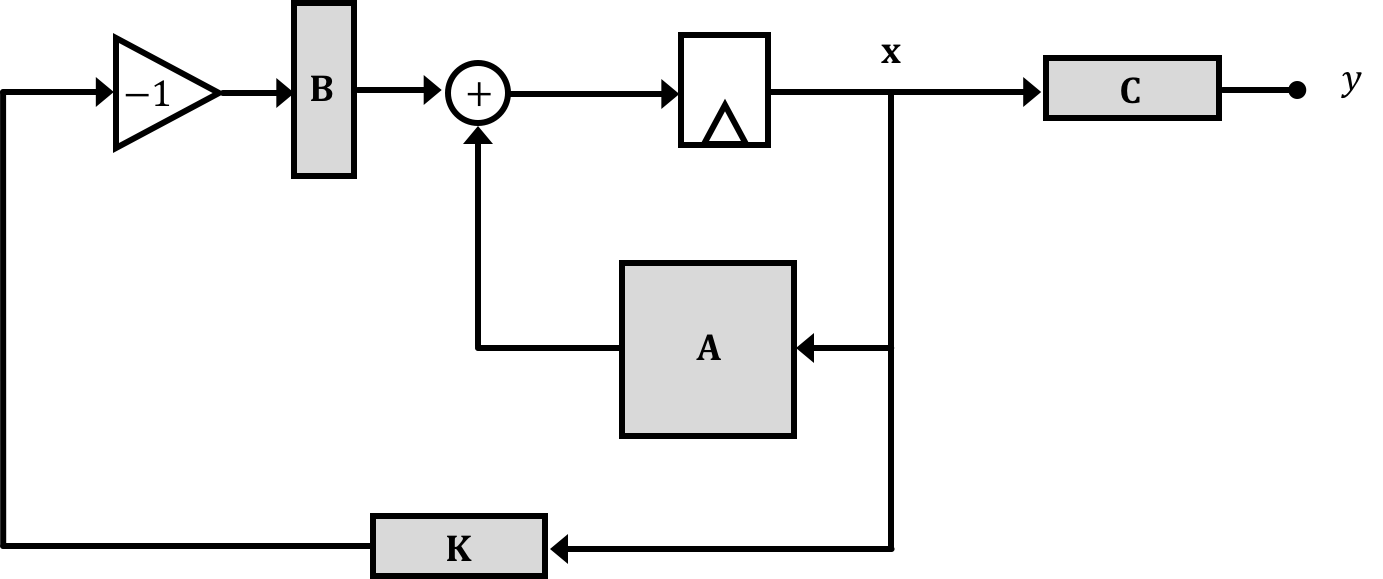
Note that this has an implied input of \(0\). Often you'll see a system with a fixed input of 0 called a regulator. We handle it exactly, the same, however the \(\textbf{B}\) the input is not longer a factor in our math so we just say: \[ \textbf{x}[n] = \textbf{A}\textbf{x}[n-1] + \textbf{B}\left(- \textbf{K}\textbf{x}[n-1]\right) \] If we distribute this out we get: \[ \textbf{x}[n] = \textbf{A}\textbf{x}[n-1] - \textbf{B}\textbf{K}\textbf{x}[n-1] \] Feedback gives us the ability to move the natural frequencies around since we're now saying that the progression of states is based not only on elements of the original \(\textbf{A}\) matrix but also the extra "paths" we've added through feedback via the gain vector \(\textbf{K}\). This means our new expression for the system natural frequencies is:
\[ \det\left(\left(\textbf{A}-\textbf{B}\textbf{K}\right)-\textbf{I}\lambda\right)=0 \]
Determine a set of gains \(K_1\) and \(K_2\) where \(\textbf{K} = \begin{bmatrix}K_1 ~~ K_2\end{bmatrix}\) to move the natural frequencies of the system in feedback so that they are both equal to \(0.9\).
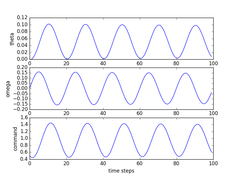
So what we just did above was put a pendulum into feedback to control the thrust applied to it using information from the states. While the (damped) system started with two complex natural frequencies, which would imply it would have a response like the following to a unit step input (where "command" is the net torque on the pendulum):
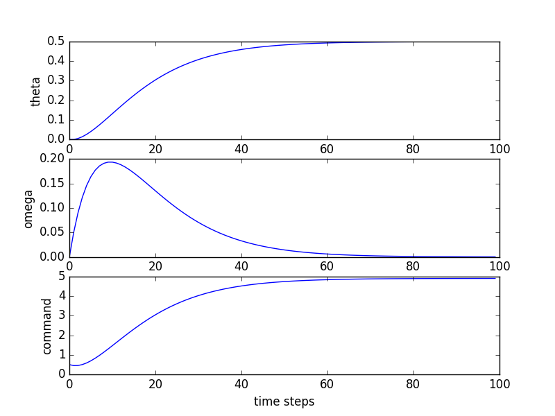
This is great! We can say, "I want these natural frequencies" and we seem to be able to get them! Well...sort of...there are some problems...It was sort of annoying to have to solve this one out by hand. It required solving for the eigenvalues of the matrix, and then selecting values of gains to move those eigenvalues around. For the \(2\times 2\) case, this isn't **too** bad, but if we were to go to \(3\times 3\) or above, it will get pretty bad and we'll need computational techniques to help us along! We'll start going into that in the next page.