State space is a very common method of analyzing and controlling systems. The idea can at first seem somewhat weird, but it is a natural progression from how we were studying and modeling systems in 6.302.0x. In this week's notes, we'll proceed to derive some basic state space formulae and discuss ways of thinking systems from the perspective of states.
The meaning of what states are is sort of odd when first introduced, but it isn't too bad or too complex when you start messing with it enough. Ideally, you've had some prior experience with coming up with system models (through deriving difference equations or transfer functions in other classes). One way of thinking of states is that they are the forms of energy that fexist within a system. Another way of thinking about it is that it is the set of system values and conditions which unambiguously predict how a system will develop over time....in other words to have a model of a system predict its behavior, you generally need to specify initial conditions. These initial conditions are generally the states (or tightly related to the states through some constants).
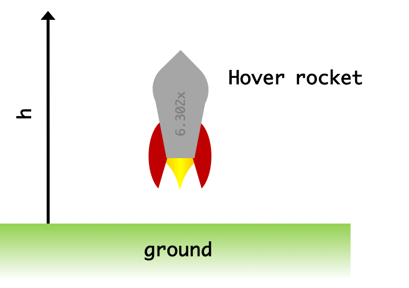
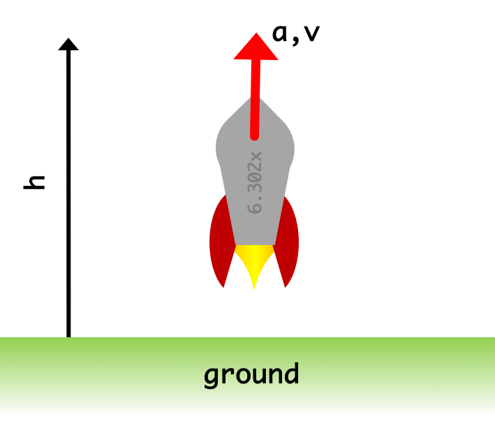
This idea is perhaps best learned and appreciated through an example, so let's consider a "hover rocket" gedanken experiment as we go through the basics of state space, where we eventually want to be able to control a second order rocket at a certain height given an ability to control the rocket's thrust (equivalent to force).
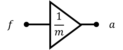
Let's assume that the input to our system is a rocket thrust, a force on the rocket from the engine burn. Stated in a different way, the control signal directly relates to acceleration using the following equation: \[ a[n] = \frac{1}{m}f[n] \] which comes from the classic \(f=ma\) of high school physics where \(f\) is force in Newtons, \(m\) is mass in kilograms, and \(a\) is acceleration in \(\text{m}\cdot \text{s}^2\).
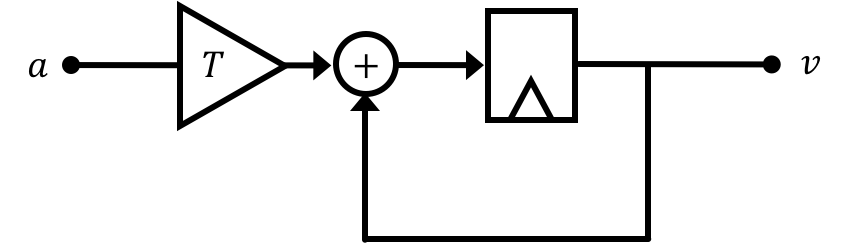
We can come up with an equation relating velocity to acceleration using what we know about integration in discrete time. Specfically we can say: \[ v[n] = v[n-1] + \Delta T a[n-1] \] Note this could also be derived from doing a forward difference discrete time approximation of a continuous time derivative, particularly: \[ a(t) = \frac{d}{dt}v(t) \approx \frac{v(T(t+1)) - v(Tt)}{T} \] Where \(T\) is the duration of our system's timesteps in seconds. Converting into discrete time notation (see 6.302.0x for review) where \(n\) is our time step number, we can say: \[ a[n] = \frac{v[n+1] - v[n]}{T} \] or after some rearrangement: \[ v[n+1] = v[n] + Ta[n] \] which can then be shifted in timesteps by one so that: \[ v[n] = v[n-1] + Ta[n-1] \] One way to think about the meaning of this equation is that the velocity on the current timestep is based on the velocity from the previous timestep plus the acceleration from the previous timestep multiplied by the duration of the timestep.
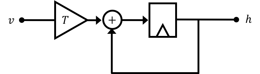
We can also come up with a similarly comprehensible equation relating velocity to height of the rocket \(h\) through a second step of integration: \[ h[n] = h[n-1] + T v[n-1] \]
With these two equations in hand we can now begin thinking about states. But before we do we're going to take a moment to refresh block diagrams since they'll help us visualize the states.
In order to help us visualize the flow of information and energy as well as how different parameters influence one another inside the system, we're also going to rely a bit on block diagrams to illustrate our systems. Aside from lines with arrows which indicate the flow of values, we'll use four main block diagram elements (bit of a 6.302.0x review here):
This block represents the multiplying of a scalar onto an value.
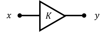
Further, it is important to remember that there is generally a direction/assignment associated with our difference equations and block diagrams. In the case of the gain block \(y[n]\) is based on \(x[n]\) not the other way around. While their algebraic relationship may still be useful in derivations, it is important to remember that as written and drawn, \(x\) causes \(y\) and not vice versa. Another way to think about the \(=\) sign here is that it is similar to the \(=\) as it is used in programming...in other words an assignment operator rathern than a statement of equality.
This symbol represents the summation of multiple signals:.
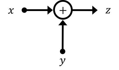
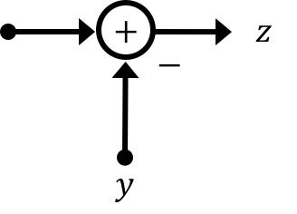
Again the \(=\) sign in these contexts should be thought of as an assignment reading right to left, so in other words in the case of the summation, \(z\) is based on the sum of the current values of \(x\) and \(y\), not vice versa.
The last symbol we'll introduce (new to both 6.302.0x and 6.302.1x to remove ambiguities with \(z\) notation) is the following:
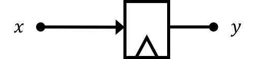
If we think about information flowing through our system, the location of delays is where information gets held up/stored on a given time step. While the other symbols and operations take place immediately (gains and summations and differences), as evidenced by the same time step on both the input and the output sides, the difference in time step here \([n]\) vs. \([n-1]\) implies a persistence and/or memory between time steps. This is critical to thinking of states.
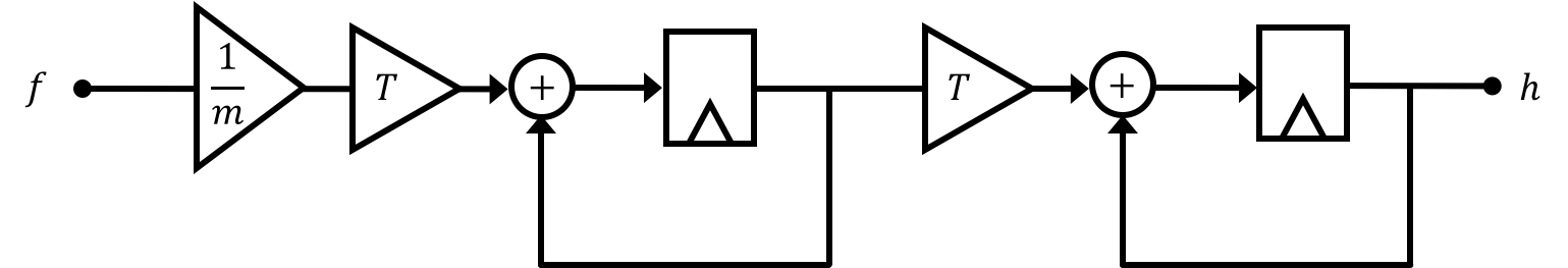
Applying our block diagrams to our hover rocket system we can generate one piece for the relationship of rocket thrust to acceleration (thrust leads immediately to acceleration):
Now at this point we should pause and think about how this system would progress over time. For simplicity let's assume \(m=1\) kg (small rocket) and \(T =1 \) second (slow microcontroller), and let's assume that we provide a unit sample input to our system \(\delta[n]\) such that: \[ \delta[n] = \begin{cases} 1\text{ if } n=0\\ 0 \text{ if otherwise}\\ \end{cases} \] What I'd like to do is calculate what the output of the system is over time, however in order to do that we need to specify what initial conditions for the system. In particular at the location of every delay block, we need to "pre-load" a value in for the start of our simulation. We indicate the two locations below for this particular model.
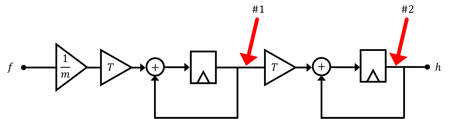
These locations have particular importance for us in this class because they can be used to identify what the states of the system are. In combination with a user-provided input, values for the two state locations below (which correspond to velocity #1 and height #2) is sufficient to unambiguously predict the system behavior.
So let's say our system starts at rest. When we say that it generally means the states of the system are set to be 0 (though this can vary depending on the situation). If we were to apply a unit sample input (again remember both \(m\) and \(T\) are set to unity), the progression of these two states and
| timestep n | Input | State 1 | State 2 | Output |
|---|---|---|---|---|
| 0 | 1 | 0 | 0 | 0 |
| 1 | 0 | 1 | 0 | 0 |
| 2 | 0 | 1 | 1 | 1 |
| 3 | 0 | 1 | 2 | 2 |
| 4 | 0 | 1 | 3 | 3 |
If we were to instead start the system with initial conditions of State 1 starting at 5 and State 2 starting at 11, and but give it the same input
| timestep n | Input | State 1 | State 2 | Output |
|---|---|---|---|---|
| 0 | 1 | 5 | 11 | 11 |
| 1 | 0 | 6 | 16 | 16 |
| 2 | 0 | 6 | 22 | 22 |
| 3 | 0 | 6 | 28 | 28 |
| 4 | 0 | 6 | 34 | 34 |
If we were to then change how the two states influence one another, by altering \(T\) so it is \(0.1), and then starting with the previous intial conditions we'd end up with:
| timestep n | Input | State 1 | State 2 | Output |
|---|---|---|---|---|
| 0 | 1 | 5 | 11 | 11 |
| 1 | 0 | 5.1 | 11.5 | 11.5 |
| 2 | 0 | 5.1 | 12.01 | 12.01 |
| 3 | 0 | 5.1 | 12.52 | 12.52 |
| 4 | 0 | 5.1 | 13.03 | 13.03 |
Again completely different. So in thinking about what states are and how to come up with them, we need to be thinking about what terms/values are needed to unambiguously describe a system.
What makes a variable a state variable? In general, if we know the input to a system for all \( t \ge \tau \), and we know the value of all the state variables at time \( t = \tau \), then we know (or can determine uniquely) the state for all \( t > \tau\). The problem, of course, is deciding which variables are state variables.
For some problems, state variable are associated with energy storage. The current through an inductor or the voltage across a capacitor are usually states, and are associated with magnetic or electrostatic energy storage. The length of a spring or the height of an object are often states, particularly if the spring is compressible or the object is in a gravity field. In the case of our rocket ship, height and velocity are the states, because once you know both at a time \( \tau \), you can determine the entire future trajectory of the rocket. It is also true that height is associated with the rocket's potential energy and velocity is associated with its kinetic energy \(E_{KE} = \frac{1}{2}mv^2\). Acceleration is not a state in this case, because it is an input to our system. In other words, while acceleration can certainly be a state, in general, but in this case, acceleration is an input to our system.
Redrawing our block diagram in a bent-back method we get the following:
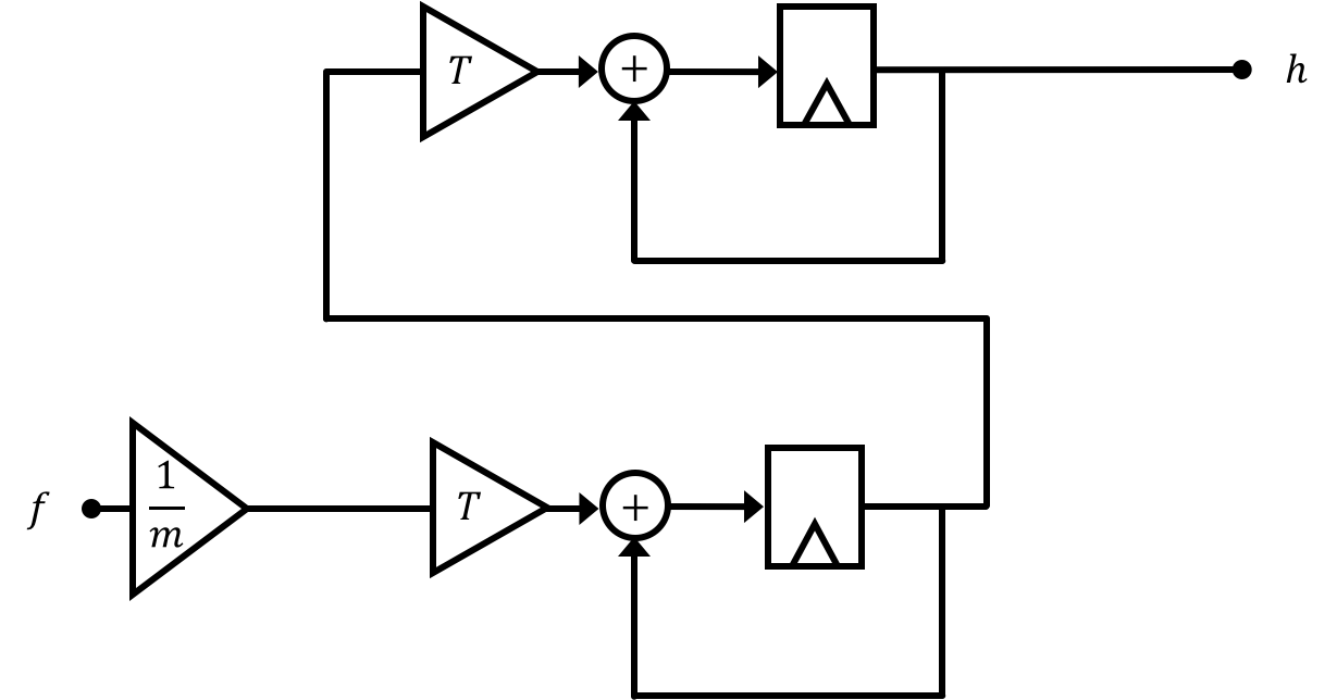
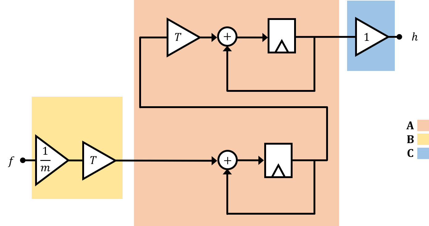
The relationship of the states to one another over time steps as well as how the system input and output are related to these states can more effectively be represented using matrices, which we will discuss on the next page.
The diagrams on the previous page might be good for when we're starting controls and for simple systems, but as we go further and the number of states goes up they will get too bulky, and hard to analyze. A solution to this problem comes from realizing that really all we're doing with those block diagrams and substitutions is linking a series of equations together. A group of equations can, when organized properly, be expressed as a matrix (that's all a matrix really is, after all...), and with this in mind we can organize how we express our relationships in the system. We'll fit these relationships into two matrix-based equations of the following form which we'll call our state space equations, where \(\textbf{A},\textbf{B},\textbf{C},\)and \(\textbf{D}\) are matrices and \(\textbf{x}\) is your state vector, \(u\) is your system input, and \(y\) is your system output. We'll use bold non-italic variables to represent matrices (to distinguish them from single variables which are italic and non-bold.:
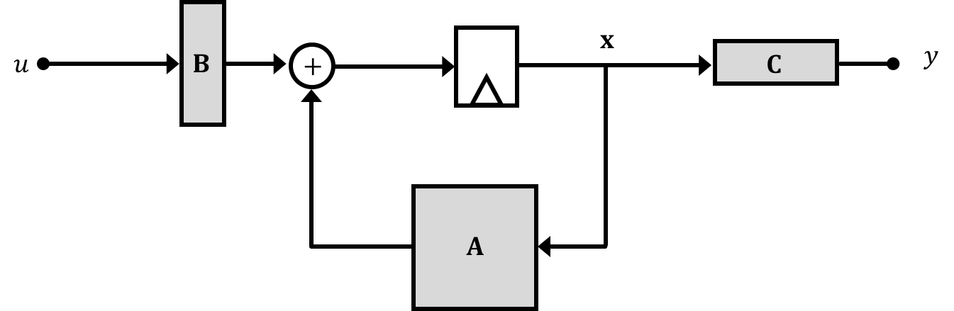
\[ \textbf{x}[n] = \textbf{A}\cdot\textbf{x}[n-1] + \textbf{B}\cdot u[n-1] \] and \[ y[n] = \textbf{C}\cdot \textbf{x}[n] + \textbf{D}\cdot u[n] \]We can represent these equations diagramatically using the following setups where grey boxes represent matrices with the shapes of the grey boxes represnt their approximate shape in a single-input-single-output system (which we're dealing with). Importantly, in these diagrams the "wires" still indicate the flow of information similar to what was discussed on the previous page, but now signals are not necessarily single values, but can instead be matrices/vectors:
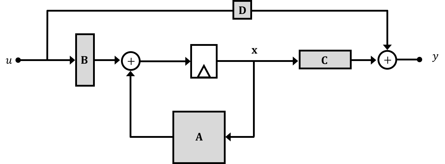
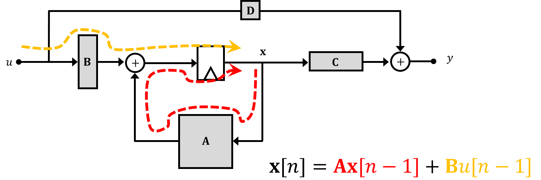
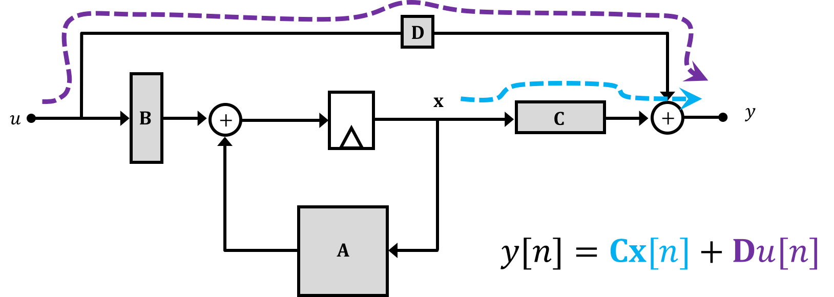
Now taken together, if we think about what this is saying, it is that the future states of the system \(\textbf{x}\) are based the current states of the system as well as current input \(u\). And the output of the system \(y\) is defined in terms of the system states at the present time.
Breaking it down by each matrix we can say:
Often (thought definitely not always!), the ability of an input \(u\) to immediately influence the output \(y\) will be negligible (usually there will be some delay and any change in input may have to propagate through the different states...in fact this disconnect between the input and output is part of the reason why we have to study controls in the first place). Therefore we'll generally ignore the \(\textbf{D}\) matrix unless we need it like so:
We said on the previous page that our hover rocket has two states which when combined along with the input to the system can be used to fully predict how the system will respond. These can also be thought of as the outputs of our delay units from the block diagrams on the previous page.
Therefore our system's state vector will be: \[ \textbf{x} = \begin{bmatrix}h\\v\end{bmatrix} \]
With our state vector defined our job now becomes fitting equations we've derived into the matrix formula above. For discrete time you want to be on the look out for equations that can be manipulated to relate future states to current states. In this initial walkthrough problem we can see pretty easily that our position and velocity equations will fit nicely. Let's generate the following: \[ \begin{bmatrix}h[n]\\v[n]\end{bmatrix} = \begin{bmatrix}1 & T\\0 & 1\\\end{bmatrix}\cdot \begin{bmatrix}h[n-1]\\v[n-1]\end{bmatrix} + \begin{bmatrix}0\\\frac{T}{m}\end{bmatrix}\cdot \begin{bmatrix}u[n-1]\end{bmatrix} \] And for a second equation where we'll just assume out output is our rocket's height we'll have the following: \[ y[n] = \begin{bmatrix}1 & 0\\ \end{bmatrix}\cdot\begin{bmatrix}h[n]\\v[n]\end{bmatrix} \] where the input has no direct effect on the output.
So now we've got this situation where: \[ \textbf{x}[n] = \textbf{A}\cdot\textbf{x}[n-1] + \textbf{B}\cdot u[n-1] \] This equation can be broken into two parts: the natural and the forced response. The natural response involves the \(\textbf{A}\) matrix and the forced response involves the \(\textbf{B}\) matrix. Focussing on just the natural (free from outside influence) behavior of the system (the homogenous equation) we get this: \[ \textbf{x}[n] = \textbf{A}\cdot\textbf{x}[n-1] \]
The solution to the homogenous equation, given the value of the initial state, \( \textbf{x}[0] \), is easy to write down, but is more difficult to interpret. That is, \[ \textbf{x}[n] = \textbf{A}\cdot\textbf{x}[n-1] = \textbf{A}^2\cdot\textbf{x}[n-2] = ... = \textbf{A}^n\cdot\textbf{x}[0]. \]
Suppose \( \textbf{A} \) where a number instead of a matrix, then we would know a lot about the behavior of \( \textbf{x}\). If that number's magnitude were less than one, \( \textbf{x}[n] \) would decay to zero, if it were bigger than one, \( \textbf{x}[n] \) would grow exponentially. And if the number was negative, or was a complex number with a non-zero imaginary part, then \( \textbf{x}[n] \) would probably oscillate. But \( \textbf{A} \) is not a number, it is a matrix, so we have no way to apply this simple intuition. Or do we?
We have one generalization from 6.302.0x. If you can express \(x[n]\) as a weighted combination of its past \( k \) values, (\(x[n-1], x[n-2], ... x[n-k] \)) then \(x[n]\) can almost always be represented as a weighted sum of powers of the \( k \) difference equation natural frequencies (as long as the natural frequencies are unique, as is usually, but not always, the case). That is, \[ x[n] = \sum_k \alpha_k \lambda_k^n x[0] \] where \( k \) is the order of the difference equation, the \( \lambda_k's \) are the (assumed unique) natural frequencies that can be computed by finding the roots of a \(k^{th} \)-order polynomial. If all the natural frequencies have magnitude less than one, \( \textbf{x}[n] \) decays to zero, if one of them has a magnitude bigger than one, \( \textbf{x}[n] \) will likely grow exponentially, and if any of them are negative, or complex, then \( \textbf{x}[n] \) will probably oscillate.
So back to powers of matrices, how do we reason about them? It turns out that something very similar to natural frequencies can be used to describe powers of a matrix. In particular, if we caste a difference equation in matrix form, then the natural frequencies are precisely the eigenvalues of the so-generated matrix \(\textbf{A}\). And the response of our system can be determined from the eigenvalues and eigenvectors of our system. So we'll still be able to utilize our knowledge of natural frequencies (magnitude greater than 1 is unstable, etc... that we learned in 6.302.0x) to inform our understanding of the system (and most importantly, to design proper control systems!!!)
\[ \textbf{A}\cdot\textbf{v} = \lambda \cdot \textbf{v} \] For solutions to the above equation, \(\textbf{v}\) is an eigenvector for the system and \(\lambda\) is an eigenvalue for the system. Quick manipulation can yield: \[ \textbf{A}\cdot\textbf{v}- \lambda \cdot \textbf{v}=0 \] and subsequently \[ \left(\textbf{A}- \textbf{I}\cdot\lambda\right) \textbf{v} = 0 \] where \(\textbf{I}\) is an \(m\times m\) matrix. such that: \[ \textbf{I} = \begin{bmatrix}1 & 0 & \cdots & 0\\0 & 1 &\cdots & 0\\\vdots &\vdots &\ddots &0\\0&0&\cdots&1\\ \end{bmatrix} \] Provided that \(\textbf{v}\) is non-zero, the above equation will have solutions only when \[ \textbf{A}- \textbf{I}\cdot\lambda \] is singular, or equivalently, when the determinant of \( \textbf{A}- \textbf{I}\cdot\lambda \) is equal to zero. So these eigenvalues end up actually being the same natural frequencies to our system that we derive in 6.302.0x.
So in returning to our original rocket problem, if we substitute our \(\textbf{A}\) matrix we get: \[ \left(\begin{bmatrix}1&\Delta T\\0&1\\\end{bmatrix}-\begin{bmatrix}1 &0\\0&1\end{bmatrix}\cdot \lambda \right)=0 \] or \[ \left(\begin{bmatrix}1&\Delta T\\0&1\\\end{bmatrix}-\begin{bmatrix}\lambda &0\\0&\lambda\end{bmatrix}\right) =\begin{bmatrix}1-\lambda&\Delta T\\0&1-\lambda\\\end{bmatrix}=0 \] Solving for the eigenvalues in this case is relatively straightforward here since the eigenvalues of the \(2\times2\) matrix are then just the determinant of the matrix so we get: \[ \left(1-\lambda\right)\left(1-\lambda\right)=0 \] which tells us that our system has two eigenvalues at \(1\). If we remember that in the case of LTI systems the eigenvalues of this system represent the natural frequencies of our system, this is telling us that the our system has two natural frequencies at \(1\). Just above, we suggest repeated natural frequencies hardly ever happen, BUT IT JUST DID. Well, it happened because our rocket model is unrealistically simple. We ignored very important forces, like air resistance, for example.
If you'd like, verify this answer, by deriving the natural frequencies the 6.302.0x way using more classical techniques! You should see the same answer show up! This is more globally known as a double-integrator system (and each integrator is giving us a natural frequency of 1), so this is a very commonly studied type of control problem!
We just showed that we can model things using a state-space approach, and there are for sure lots of benefits of doing this, but the real power of state space comes when you start to use it for control.
In 6.302.0x where we work up Proportional+Difference and Proportional+Integral+Difference controls which are based on the idea of applying varying gains to "error" signals based on the comparison of desired output to actual output in order to drive our plant towards a state we desire, state space allows us to instead feed back our states and apply gains to them as shown below.
The idea here is that we can use the values of our states to adjust our input, just like we do in the more traditional idea of feedback that is covered in 6.302.0x, but instead of being limited to just signals based on input-to-output error (or the derivative/difference or integral) we can potentially use all the states of the system.
For starters, we begin by considering a vector of state-feedback gains, denoted \(\textbf{K}\). For a system with \( m \) states, \( K \) could be a \(1 \times m\) row vector such that when multiplied by our state vector, an \(m \times 1\) column vector, results in a scalar value: \[ \textbf{K} \textbf{x} = \begin{bmatrix}K_1, K_2,\ldots,K_m\end{bmatrix} \cdot \begin{bmatrix}x_1\\x_2\\\vdots\\x_m\end{bmatrix} = \sum_{i=1}^m K_i x_i. \]
Now what would happen if we take this resulting scalar and tie it in with negative feedback to a different input signal \(u'\) like shown below (NOTE THIS \(u'\) IS NOT THE SAME AS \(u\) FROM BEFORE. WE'LL DISCUSS THIS IN A BIT).
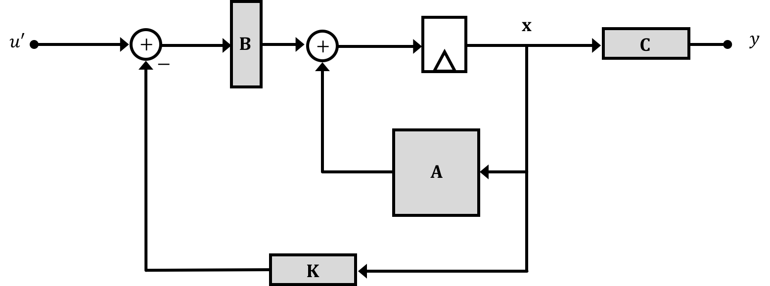
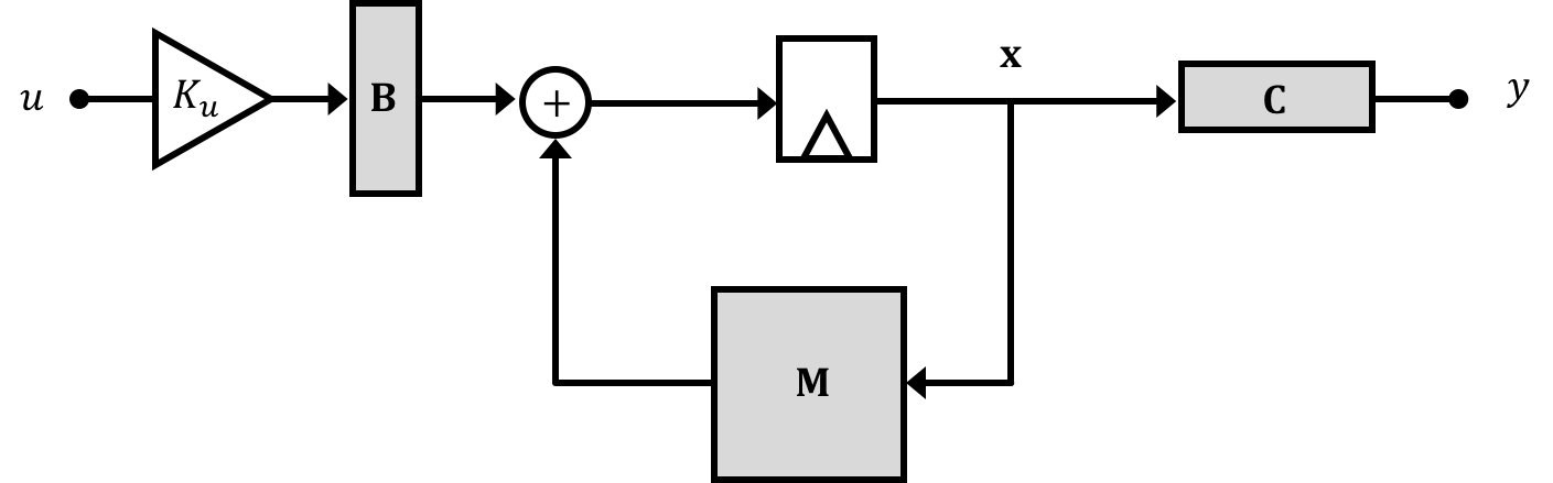
Now, before the system's behavior could be taken to be a power series based on the natural frequencies which were in turn the eigenvalues of the matrix \(\textbf{A}\), the system now can be thought to have a modified feedback matrix (it isn't just \(\textbf{A}\) anymore!!). We'll call this matrix \(\textbf{M}\) so that: \[ \textbf{x}[n] = \textbf{M}\cdot\textbf{x}[n-1] \] where \[ \textbf{M}=\textbf{A} - \textbf{B}\textbf{K} \]
With no feedback \(\textbf{M} \to \textbf{A}\), but with feedback we can potentially change the form of our feedback \(\textbf{M}\) matrix which in turn will change the eigenvalues of the system which will in turn change the natural frequencies of the system which is what we hope to accomplish since this can provide us a path towards adjusting the response of a system/stabilizing it!
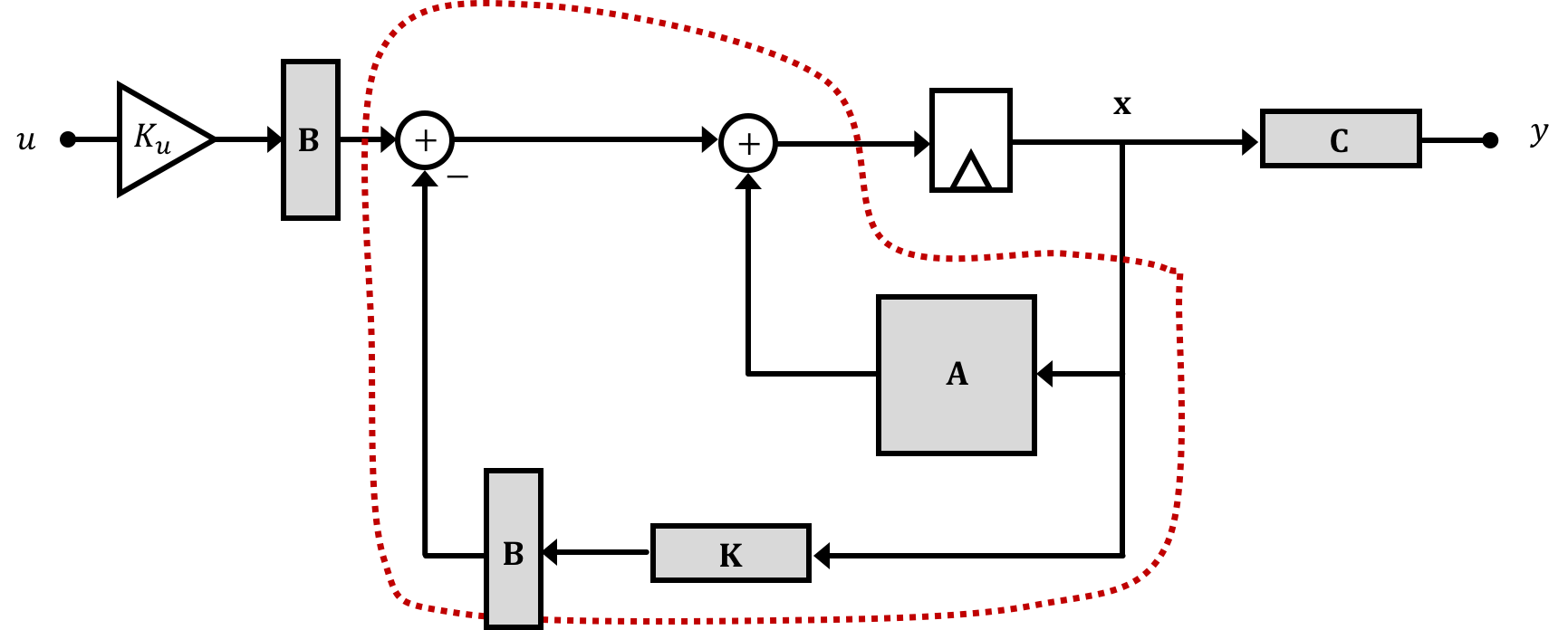
In fact if we distribute our \(B\) matrix out prior to the subtraction at the input of our system we can then clearly see that we can lump together a portion of our state-feedback system outlined by the dotted maroon line below...
So what this says is that state feedback is a means of changing the eigenvalues of a system towards a specific end. Just like in 6.302.0x where we pick gains like proportional and difference gain (\(K_p\) and \(K_d\), respectively, which bring our system's natural frequencies within the unit circle (magnitude less than 1) or make them purely real (avoid oscillation) to produce desired behaviors, by picking values of our state feedback vector \(\textbf{K}\) we can achieve the same thing and the affect can often be more readily apparent!
Ok we just saw how the addition of state feedback provides the means of changing the system's natural frequencies (eigenvalues), but there is one more change we need to make before we can start applying this systems. In the previous section we made a derivation with a modified input signal \(u'\) and the reason for the information generated and fed back to our plant input cannot be directly combined with our input. Instead what we must do is add an input scalar which we'll call \(K_u\) right at the beginning of our system in order to make things work out. Diagramatically this looks like the following:
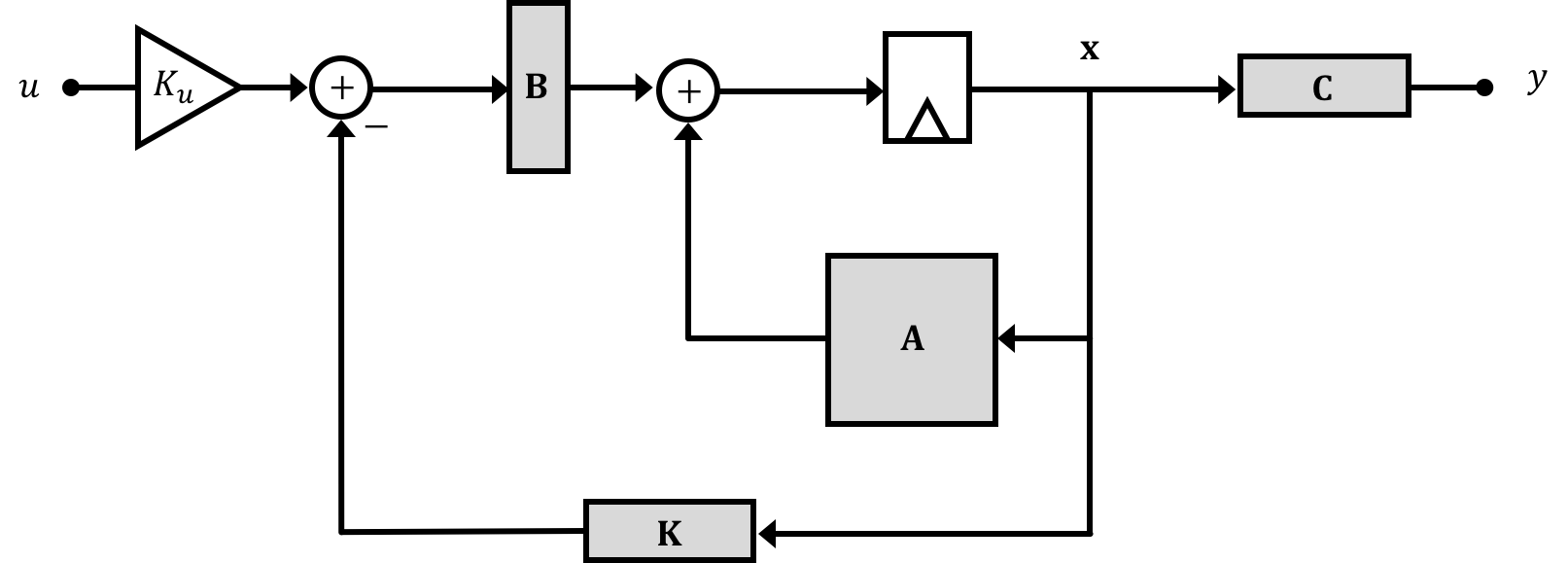
Determination of an expression and/or value for \(K_u\) is a relatively easy derivation. If we assume the system can reach a steady-state value (that is that we can modify its natural frequencies via feedback to have it converge on a stable set of states), when the system reaches steady state we can say that \(\textbf{x}[n+1] = \textbf{x}[n]=\textbf{x}[n_{\infty}]\) where we use the subscript \(\infty\) to represent timesteps far in the future after the system has stabilized (very large \(n\) or as \(n\to \infty\)). This is basically saying that from time step to time step the states will not be changing, which if we're dealing with a constant input (relative to system dynamics) is exactly what we want. This equality allows us to modify our primary state space equation so that: \[ \textbf{x}[n_{\infty}] = \left(\textbf{A}-\textbf{B}\cdot\textbf{K}\right)\textbf{x}[n_{\infty}] + \textbf{B}K_uu[n_{\infty}] \] which we can rewrite as: \[ \left(\textbf{I}-\textbf{A}+\textbf{BK}\right)\textbf{x}[n_{\infty}] = \textbf{B}K_uu[n_{\infty}] \] and then finally as: \[ \textbf{x}[n_{\infty}] = \left(\textbf{I}-\textbf{A}+\textbf{BK}\right)^{-1}\textbf{B}K_uu[n_{\infty}] \] Substituting this into our state space system's output equation: \[ y[n] = \textbf{C}x[n] \] we can say: \[ y[n_{\infty}] = \textbf{C}\cdot \left(\textbf{I}-\textbf{A}+\textbf{BK}\right)^{-1}\textbf{B}K_uu[n_{\infty}] \] Since we'd ideally like our system's output \(y\) to track our input \(u\) we'd therefore like \[ \frac{\textbf{y}[n_{\infty}]}{u[n_{\infty}]} = 1 = \textbf{C}\cdot\left(\textbf{I}-\textbf{A}+\textbf{BK}\right)^{-1}\textbf{B}K_u \] So we can come up with an expression for the input scaling term \(K_u\) \[ K_u = \left(\textbf{C}\left(\textbf{I}-\textbf{A}+\textbf{BK}\right)^{-1}\textbf{B}\right)^{-1} \]
Therefore the takeaways from this are that given a state space model with \(\textbf{A}\), \(\textbf{B}\), and \(\textbf{C}\) matrices we can possibly pick feedback gains contained within a matrix \(\textbf{K}\) that are applied to our states and in conjunction with our system input (scaled by \(K_u\)) we can work towards controlling our system.
So let's return to our hover rocket problem. Let's say we had the following \[ y[n] = h[n] \] Remembering the system of equations from the hover rocket problem: \[ \begin{array}{lcl} h[n] & = & h[n-1]+Tv[n-1] \\ v[n]& = & v[n-1] + Ta[n-1] \end{array} \] We define our state vector to be \[ \begin{bmatrix}h[n] \\ v[n]\end{bmatrix} \]
With our state vector defined our job now becomes fitting equations we've derived into the matrix formula from the previous section. For discrete time you want to be on the look out for equations that can be manipulated to relate future states to current states. In this initial walkthrough problem we can see pretty easily that our position and velocity equations will fit nicely. Let's generate the following: \[ \begin{bmatrix}h[n+1]\\v[n+1]\end{bmatrix} = \begin{bmatrix}1 & T\\0 & 1\\\end{bmatrix}\cdot \begin{bmatrix}h[n]\\v[n]\end{bmatrix} + \begin{bmatrix}0\\\frac{T}{m}\end{bmatrix}\cdot u[n] \] And for a second equation where we'll just assume out output is our rocket's height we'll have the following: \[ y[n] = \begin{bmatrix}1 & 0\\ \end{bmatrix}\cdot\begin{bmatrix}h[n]\\v[n]\end{bmatrix} \] where the input has no direct effect on the output.
If we were to place this system into state feedback and set it up so that we have some feedback gain on the term corresponding to \(h[n]\) what form of control will be implementing?
What we'd like to do is implement state feedback generally on our hover rocket problem with the initial goal here of implementing proportional control. Solving this out we'll say our new matrix is the following: \[ \textbf{M} = \textbf{A} - \textbf{B}\cdot\textbf{K} \] and let's say: \[ \textbf{K} = \begin{bmatrix}K_p & 0\\\end{bmatrix} \] where we're picking \(K_1\) to be a term \(K_p\) since we'll use that in proportional feedback. (it interacts with the angle of the arm). Evaluating for \(\textbf{M}\) results in the following: \[ \textbf{M} = \textbf{A} - \textbf{B}\cdot\textbf{K} = \begin{bmatrix}1 & T\\0 & 1\end{bmatrix} - \begin{bmatrix}0\\\frac{T}{m}\end{bmatrix}\cdot\begin{bmatrix}K_p &0\end{bmatrix} \] which then works out to be: \[ =\begin{bmatrix}1 & T\\0 & 1\end{bmatrix} - \begin{bmatrix}0&0\\\frac{K_pT}{m}&0\end{bmatrix} \] So \[ \textbf{M} = \begin{bmatrix}1 & T\\-\frac{K_pT}{m} & 1\end{bmatrix} \] We can then solve for the eigenvalue for this matrix \(\textbf{M}\) to see what the new natural frequencies are. For the sake of transparency, we'll do that here, but as we work with larger matrices we'll rely upon Python to do this for us (see software notes).
Solving for the eigenvalues of the system we'll end up with: \[ \begin{bmatrix}1-\lambda & T\\-\frac{K_pT}{m} & 1 - \lambda \end{bmatrix} = 0 \] which provides a characteristic equation of: \[ \left(1-\lambda\right)^{2} + \frac{K_{p}T^{2}}{m} = 0 \] Expanding we get: \[ 1+\frac{K_{p}T^{2}}{m}-2\lambda+\lambda^{2}=0 \] and when we solve for \(\lambda\) we get two solutions: \[ \lambda_{1,2} = 1 \pm T\sqrt{-\frac{K_{p}}{m}} \]
This is interesting since the result is telling us our closed loop system results in two natural frequencies, both of which will have a magnitude greater or equal to 1 regardless of the value chosen for \(K_p\). For those of you who have gone through 6.302.0x, this result should look familiar. The hover rocket system is second order "double integrator" system, and it is not going to be stabilizable with just proportional control.
If we go ahead and then analyze our expression for \(K_u\) we'll see the following: \[ K_u = K_p \] And this is interesting, but also of relatively little meaning since the \(K_u\) derivation above, assumed the system was able to reach a steady state via a stable response, and we weren't able to do that here.
Doing out matrix algebra can be fun at times, but when it stands between you and an answer, repeatedly doing it out manually can quickly get annoying. It is for this reason that computational devices are very useful.
Since you already have Python installed, we recommedn you install sympy library, which can be done by:
pip install sympyor in the case of Python3 (recommended) installed alongside a Python 2.7 flavor:
pip3 install sympyWith this you can create symbolic matrices and perform math as needed. For example, in our proportional control case above, the following Python script can be used to generate the outputs:
from sympy import *

T = Symbol('T') #create 'T' symbol
m = Symbol('m') #create 'm' symbol
Kp = Symbol('Kp') #create 'Kp' symbol

A = Matrix([[1,T],[0,1]]) #A matrix
B = Matrix([[0],[T/m]]) #B matrix
C = Matrix([[1,0]]) #C matrix
K = Matrix([[Kp,0]]) #K matrix

print("Open Loop Natural Frequencies/Eigenvalues:")
print(A.eigenvals())
print("Closed Loop Natural Frequencies/Eigenvalues:")
M = A- B*K #calculate closed loop state transition matrix
print(M.eigenvals())
print("Ku Value:")
Ku = (C*(eye(2)-A +B*K)**(-1)*B)**(-1) #calculate input scaling gain
print(Ku)
If we were to assign values of \(m=10000kg\) and \(T = 0.01s\) to our system, what would the natural frequencies of the hover rocket be without any feedback?
We note that the original matrix that governs the rocket without feedback is \(\begin{bmatrix}1&T\\0&1\end{bmatrix}\). Finding the eigenvalues of that we see: \[ \begin{bmatrix}1-\lambda & T\\0 &1-\lambda\end{bmatrix} \] Thus we find that we have the characteristic equation: \[\left(1-\lambda\right)^2=0 \] And therefore: \[ \lambda_{1,2}=1 \]
If we were to assign values of \(m=10000kg\) and \(T = 0.01s\) to our system and placed the system into a state feedback configuration (implementing proportional control) such that \[ \textbf{K} = \begin{bmatrix}K_{p} \\ 0\end{bmatrix} \] where \(K_p = 5\), what would the natural frequencies of the hover rocket be?
We learned earlier that this matrix is the proportional feedback matrix for the rocket: \(\begin{bmatrix}1&T\\-\frac{K_pT}{m}&1\\ \end{bmatrix}\). Solving the characteristic equation of this we find: \[ \lambda = 1\pm T\sqrt{-\frac{K_p}{m}} \] Substituting the values given we find that our two natural frequencies are: \[ \lambda_{1,2}=1-0.0002236j,1+0.0002236j \]
If we were to assign values of \(m=10000kg\) and \(T = 0.01s\) to our system and placed the system into a state feedback configuration (implementing proportional control) such that \[ \textbf{K} = \begin{bmatrix}K_p\\K_d\end{bmatrix} \] where \(K_p = 50\) and \(K_d=10\), what would the natural frequencies of the hover rocket be?
Solution: Using the new \(\textbf{K}\) matrix and solving the characteristic equation we find that \[ \lambda_{1,2} = \frac{-K_dT+2m}{2m} \pm \frac{T\sqrt{K_d^2-4K_pm}}{2m} \]
So we've introduced the idea of state space. We'll proceed to dig deeper into this in the coming weeks, and investigate the implications and benefits of it. For Lab 01, you'll derive and implement a state space controller to recreate proportional+difference control in our propeller system.