There are two key ideas in this second lab:
One can design an arm position controller by first constructing a state-space model of the system, then selecting desirable pole locations, and finally using a program like acker to determine the state-feedback gains. When you try to use this approach, you are likely find it hard to pick good pole locations, and many seemingly-good choices lead to overly large gains.
For many nonlinear systems we can use a linear state-space model, like with\( \textbf{A},\textbf{B},\textbf{C},\textbf{D} \) matrices, but only when we try to describe variations from a nominal state. Managing the offsets associated with the nominal state (the arm in the horizontal position in our case) requires some care.
acker to numerically determine gains for the full-state feedback control scheme. If you have not read through the Week 2 notes first, make sure to do that since we'll assume you've already installed the appropriate Python libraries.
The design process you'll undergo is going to be a bit more open-ended than what you may find in another lab...there will be no one right answer. In particular, depending on how your system is implemented (if you deviated much from the depicted construction), you may find that you need to adjust system parameters and constants which are included. In fact even if you built the system exactly as we specified, you may find that the gains returned by the numerical methods may not work very well. This is how it sort of should be! Our model makes a lot of assumptions, and also doesn't deal with the problem of noise, and so what comes out of the model should be used as a guide, but perhaps not an answer as to what gain values should be used!
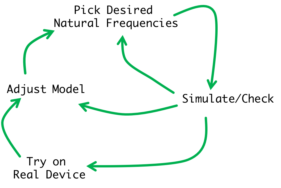
While experimenting with your simulation and gains and system, remember that this is an iterative process and what you get the first time through the cycle will probably not be good. Repeated trial-and-error cycles will be beneficial:
And as mentioned above, we will also address a second issue. In our three-state model for the copter-levitated arm, the states are: arm rotational velocity, \( \omega_a \), arm angle, \(\theta_a \) and the motor rotational velocity, \( \omega_m \) (with \( \omega_m\) represented by motor back-EMF, \( v_{emf} \)). When we model the system with \( \textbf{A},\textbf{B},\textbf{C},\textbf{D} \) matrices, we are assuming linearity, even though we know the system is nonlinear. What we are relying on is approximate linearity when we consider small displacements from horizontal, but we will have to determine how best to remove the offset in motor speed needed to acheive the horizontal position.
In looking forward, what we can learn about our model will also be able to help us next week in Week 3, as we use better tools to determine gains (the LQR approach, and also use an observer to estimate our system's states rather than trying to extract them manually from our measurements.
At the top of the code, we include a list of system parameters, such as moments of inertia, How did we come up with some of these parameters?
We approximated the moment of inertia of the propeller \(J_m\) as that of a flat rod rotating around its center. This moment is expressed using this equation: \[ J_m = \frac{1}{12}m\left(l^2+w^2\right) \] In the case of our propeller it works out to be: \[ J_m = \frac{1}{12}\cdot 0.003\text{kg}\cdot\left(0.13^2 +0.015^2\right)\approx 3\times10^{-6}\text{ kg}\cdot\text{m}^2 \]
We approximated the moment of inertia of our arm assembly as that of a narrow rod on an axis and a point mass summed together. Therefore: \[ J_a \approx J_{rod} + J_{pm} = \frac{1}{3}m_{arm}l_{arm}^2 + m_{prop}l_{arm}^2 \] Based on our measurements we got a value of about \(J_a = 4.5\times 10^{-4} \text{kg}\cdot \text{m}^2\).
We calculated a number of motor parameters through a series of experiments briefly detailed below. I'm including a writeup on how we did this in case you want to do something similar (don't feel obligated) for this setup or in the context of other systems!:
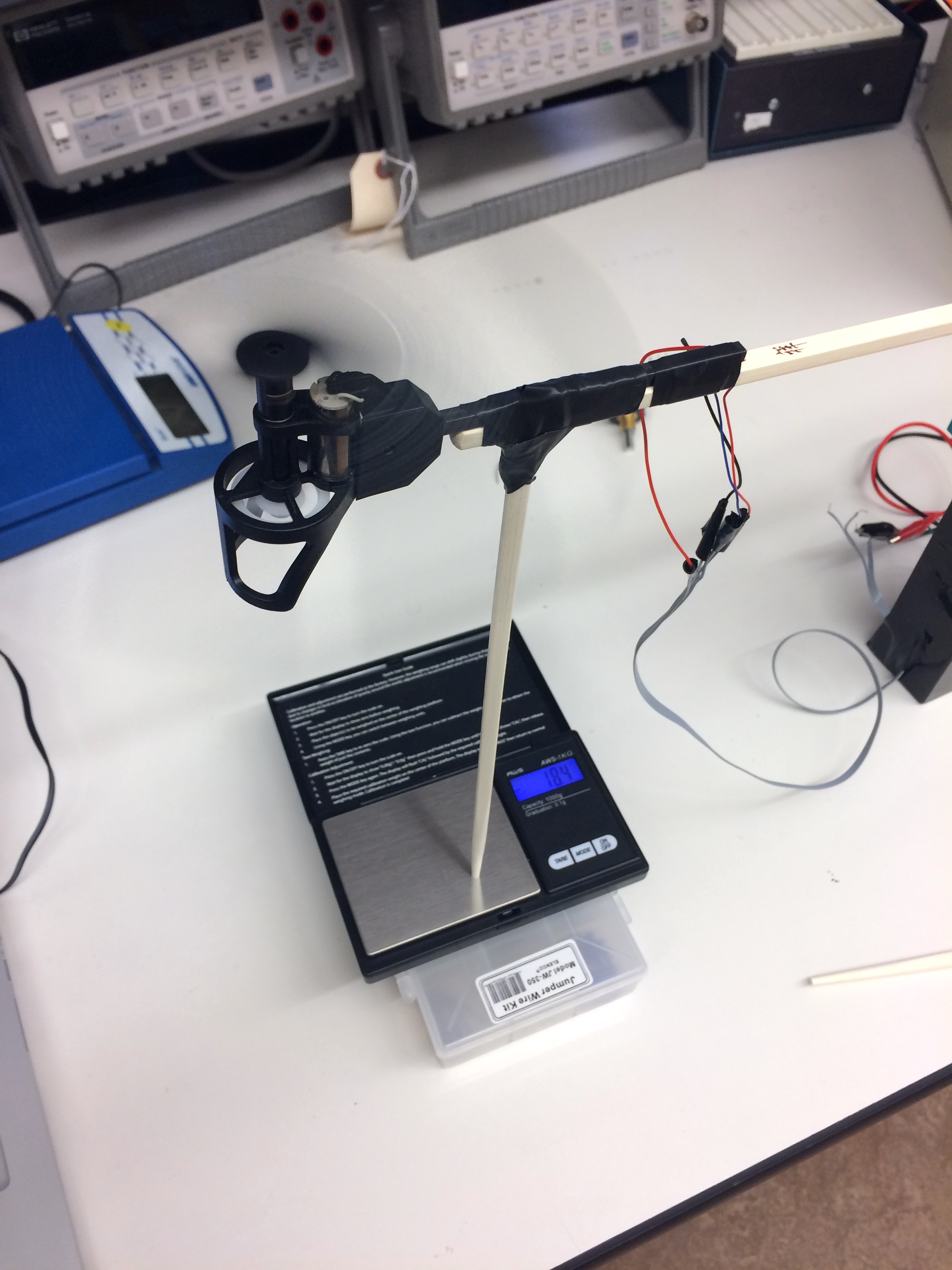
We first mounted the propeller assembly on a scale and zeroed the weight when it was not running like shown below. We then proceeded to gradually increase the voltage applied to the motor while tracking the current through the motor as well as the change in sensed mass on the scale
The motor's electrical resistance \(R_m\) was measured in two ways. First we just took an Ohmmeter and attached read the resistance. Additionally, we found a slightly different value by incorporating the motor into a circuit with a number of other low-value fixed resistors, and then by measuring the voltage drop across parts of the circuit could back out a value of approximately \(R_m\approx 0.5\Omega\).
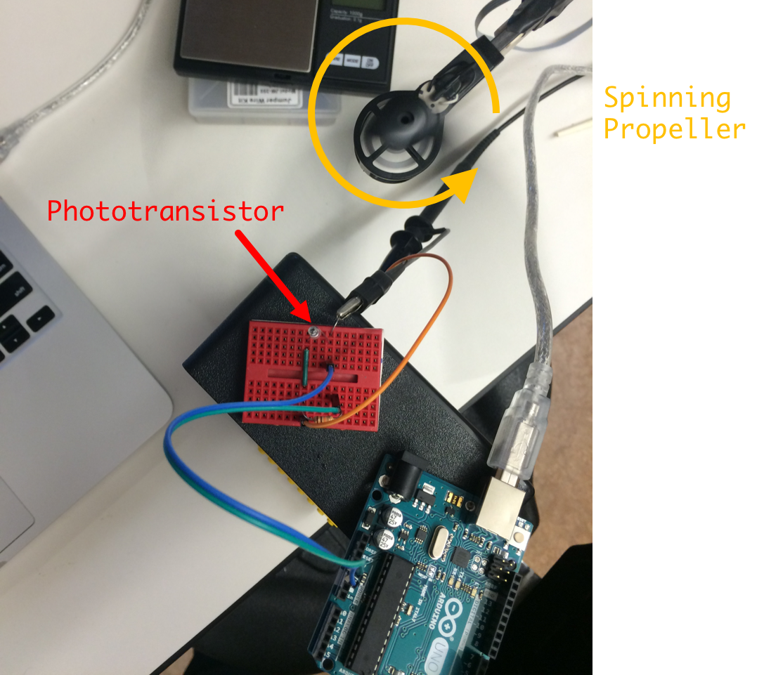
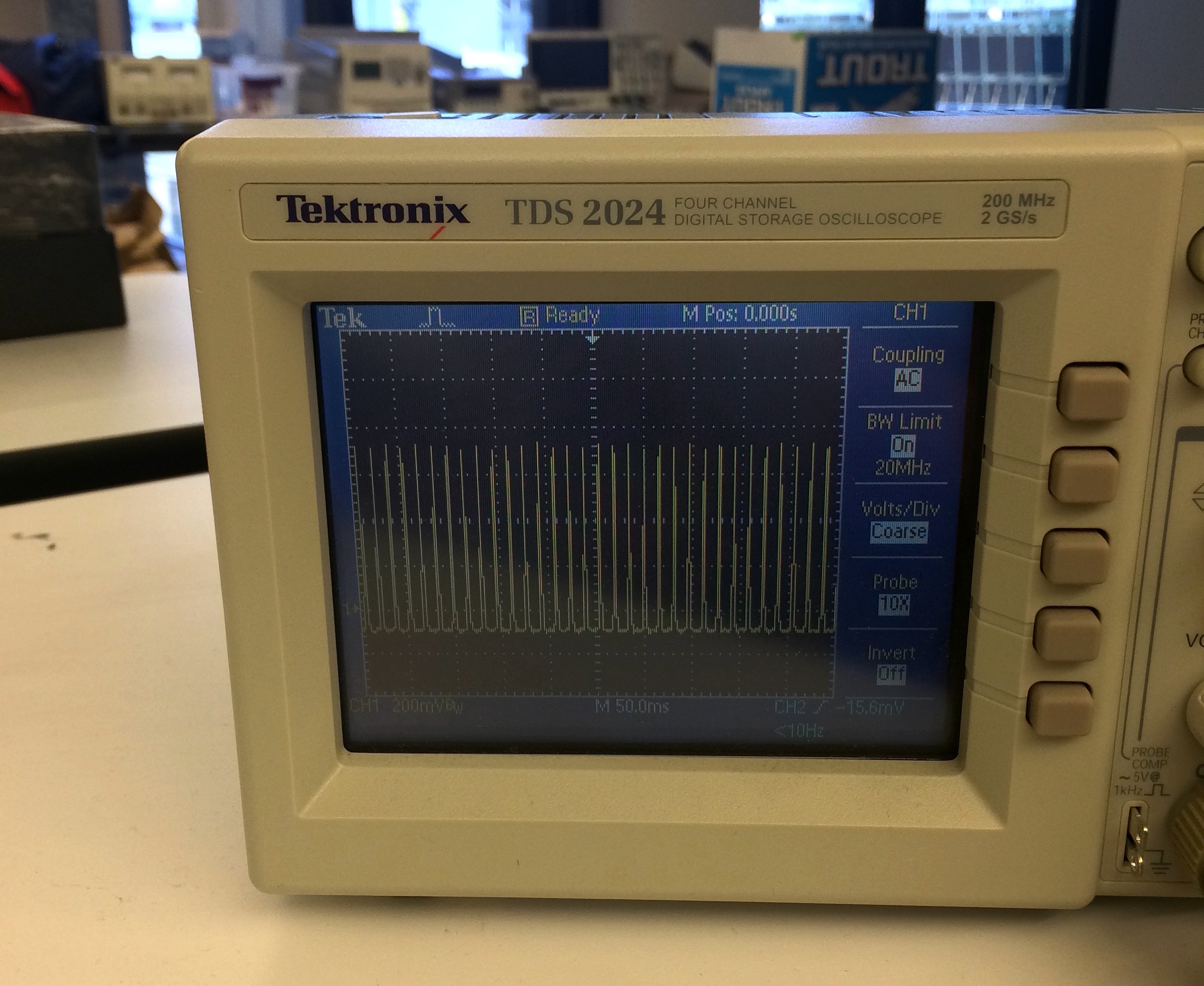
The Back EMF of the motor was relatively easy to calculate once we had a resistor value \(R_m\) to work with. What was trickier to do was determine the back EMF coefficient \(K_e\). For that we need to know the motor's angular velocity \(\omega_m\) as a function of current or voltage or something and we figured that out by building a cheap phototransistor-based (Digikey part number 1080-1152-ND in case you're interested) optical sense-circuit placed immediately below the propeller while it was running. By monitoring the output of this simple circuit on an oscilloscope we could use the deviation in signal (generated by room light being "chopped" by the rapidly passing propeller blade) to get real time measurements of the motor speed.
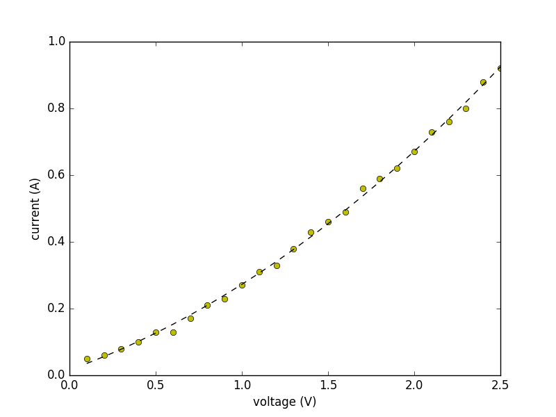
With data collected we could start coming up with relationships between parameters measured. We found the relationship between the motor voltage and the current through the motor to be roughly quadratic in shape (data points are yellow dots and fitted curve is black dashed line):
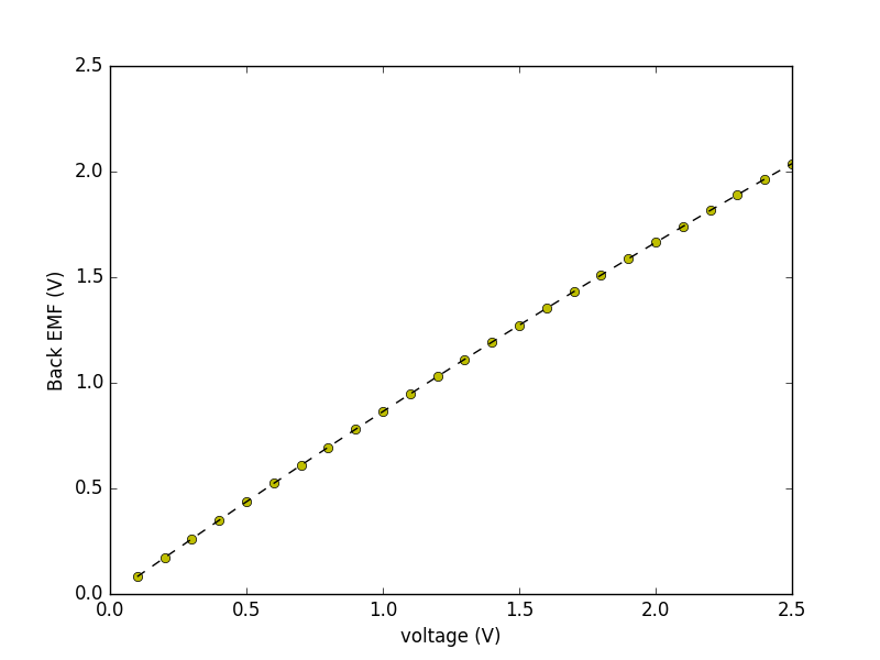
Since we already had a rough idea of the coil resistance (\(R_m \approx 0.5\Omega\)), we could use this curve to come up with an expression for the back EMF as a function of applied voltage by saying (review our simplified motor model from week 1): \[ v_{emf} = v_m - i\left(v_m\right)0.5 \] When we plot our fitted function using this modifiation we end up with the following new fitted equation:
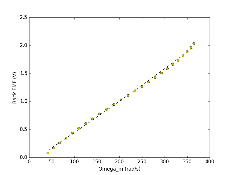
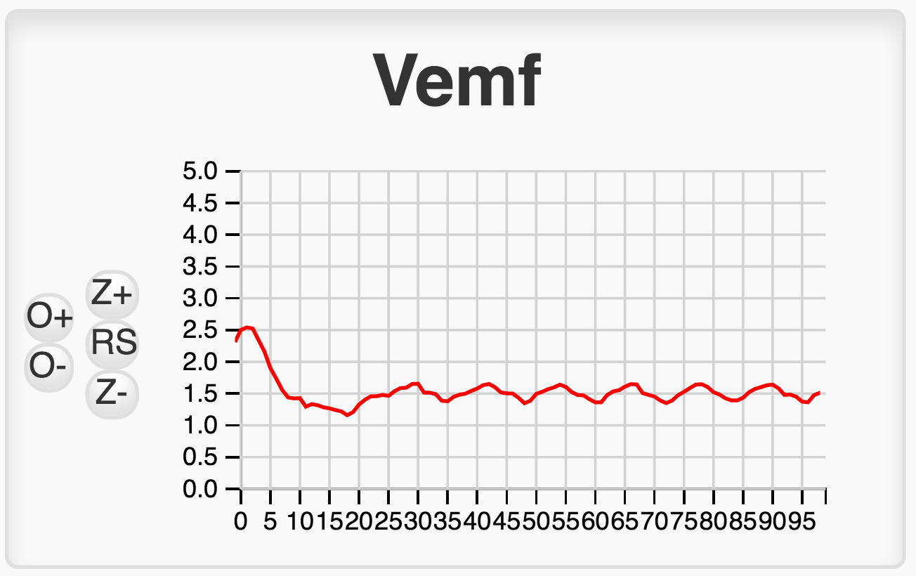
Now we need to figure out if our relationship between back EMF and propeller speed \(\omega_m\) is linear. To do this we can plot data points of calculated back EMF (figured out above) for a given voltage compared to measured propeller speed for that same given voltage. When we do this we get the following plot (data in yellow, fitted curve in black dashed):
We also made the assumption that the back emf coefficient (\(K_e\)) is equal to the motor torque coefficient \(K_m\), which is often done for motors so \(K_m = 0.0053\) as well!
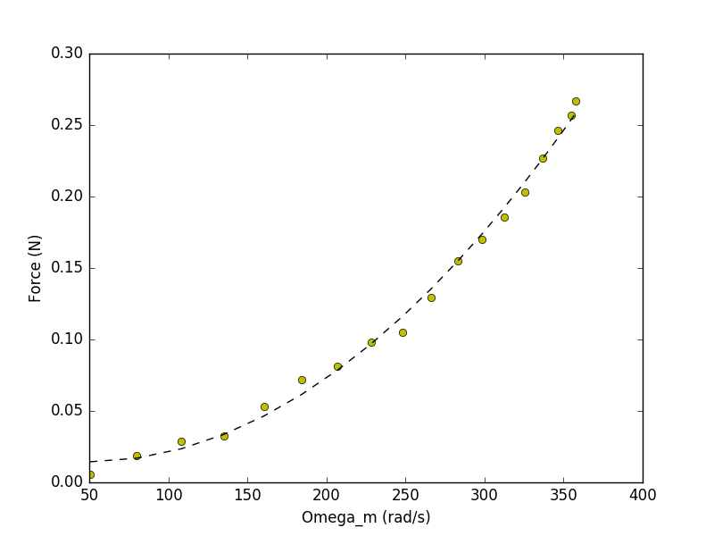
The last critical term that we're missing is the relationship between motor speed \(\omega_m\) and the thrust generated by the propeller. We expect this thrust to be proportional to the square of our motor speed and when we plot those two values out we get the following set of data points (yellow):
OK we have some parameters!
The Teensy Code for the lab can be found here (TEENSY CODE) and the basic Python skeleton for numerical calculation of gains and simulations can be found here (PYTHON CODE).
The Teensy code is not changed much from last week, with the exception that the lab02 file ships with a functioning headroom value (minor backend information for Jacob and Joe) and as it set up to already be plotting Back EMF (\(K_e\omega\)) as a state rather than motor speed \(\omega\). Therefore make sure you have the properly impelemented motorCmd line in this new version!
The Python code "skeleton" comes to you in a form very similar to what you saw in the Week 2 notes:
discrete lqr that we can use down below.acker or lqr Keep in mind that in the simulation, both angle \(\theta_a\) and angular velocity \(\omega_a\) are running in radians rather than the degrees which we have plotted in the GUI. There is a variable right above the plotting section that will scale the \(\theta_a\) and \(\omega_a\) plots so that they are in degrees instead if you want that. Run a couple simulations and see what pops out!
Your first task is to implement a Python-based model of our system by filling in the appropriate \(\textbf{A}\), \(\textbf{B}\), \(\textbf{C}\), and \(\textbf{D}\) matrices. Go back to Lab 01, review the derivations made there and build your state space model up. Note there are several parameters included in the code that are set to 0 (the friction coefficient of the motor, the drag imparted on the motor resulting from arm movement) that you should feel free to manipulate.
Once you've built your model, begin to use manual placement of the gains, as well as computational tool acker in order to pick gains. Use the resulting plots as a guide about whether or not these particular gains could result in reliable behavior. From there, then consider either implementing on the actual system, or consider adjusting your model!
You have two choices for how to deal with the offset in back EMF. That is, you will need the motor to spin at a certain speed to give you enough thrust to hold the arm at the nominal horizontal position. If you do not address the issue, you will notice as soon as you bring in a significant amount of gain on the back EMF term, the arm will droop. You may have also noticed that in our model derivation that we neglected gravity, because we assumed it would be exactly balanced by the thrust produce by the motor when it obtains the nominal value of back-EMF. Things work out by adding in a direct term to effectively "offset" gravity and let us use our model a bit more. That works at least when we're basing our feedbabck only upon the \(\theta_a\) and \(\omega_a\) terms. Once we start including \(\omega_m,\) this starts to break down.
The reason for this is that in our code the variable motor_bemf which is used to hold the measured motor back EMF does not actually contain the same quantity as is expressed in our \(\omega_m\) state in the Python simulations. To explain this further, notice in the plot below of our three system states and the control input over time how all three system states ultimately go to \(0\):
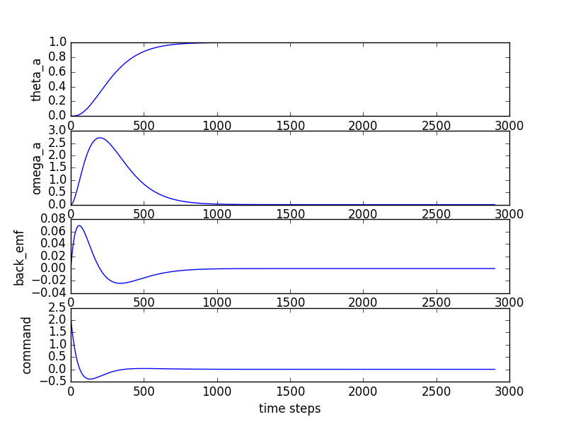
In fact, you can see that the noise/oscillations aside, the nature of the real-life plot to the Python simulation plot can be potentially look very qualitatively similar, but that the real-life one is always offset by a roughly constant amount compared to the value in the Python simulation. The reason for this is the directV we have in the code, and which you specify through the "Direct" slider. In that code our back_emf term is really being generated with the following:
\[
\texttt{back_emf}[n] = K_e\omega_m[n] + K_e\omega_{mss}
\]
where \(K_e\omega_m[n]\) is the term from our Python simulation and \(K_e\omega_{mss}\) is the term that results from adding a gravity-offset value to the directV variable (through its matched GUI slider). Now at some point in your code (if you implemented it correctly we are you will be doing the following (pseudo code warning!):
motorCmd = directV -... K3*back_emf;
If the value contained within back_emf is too large because it contains the gravity-canceling offset term \(\omega_{mss}\) we can expect that for a given value of \(\omega_m[n]\) we'll end up subtracting off too much! And we're seeing just that! As you increase your \(K_3\) gain, you do indeed see your propeller arm drop down (with all other terms being held constant!).
So how could we fix this? One solution could be to determine, by experiment, the steady-state value of back-EMF to hold the arm horizontal, and then subtract that value from the motor_bemf term. To run the experiment, we will have to adjust the gains associated with proportional and delta feedback in order to stabilize the arm, then we can adjust the direct term until the the arm is horizontal, and then we can record the value motor_bemf. Finally, we can subtract that number from the motor_bemf term before applying the gain, as in motorCmd = directV -... K3*(motor_bemf - motor_bemf_offset);.
A second, arguably easier way to fix this problem is to adjust the \( K3 \) gain, then readjust the \( direct \) value to bring the arm back to horizontal, and then test the performance of the controller. But, then WE MUST BE DISCIPLINED about readjusting the direct term every time we change \( K3 \). It is easy to forget, and if you do, you will come to incorrect conclusions.. To implement such a strategy in real time, set up your arm so that it is approximately level by adjusting the "Direct" term. Then add in all the gain terms (including \(K_u\)) using the sliders. Finally add in more "Direct" to bring the system back to level. This should hopefully remove any offsets, including those that come from the non-steady-state back EMF value!
Simulations rarely fully capture a system's behavior. Little differences like what we just explored are extremely important to keep track of. Not realizing what the signals vs. additional real-life terms, can cause huge amounts of headache!
Study what the difference in system response is for a given set of generated gains \(\textbf{K} = \begin{bmatrix}K_1 & K_2 & K_3\end{bmatrix}\) when you keep or remove the \(K_3\) term.
Depending on how your experiments go, your results may either be really good or not as good as you'd like. But most likely, you will decide that you need a better approach for determining gains than guessing where the poles should be, and using acker . Next week, we will learn about LQR, and see that it is not a perfect tool for designing controllers, but makes getting good gains far easier.