We're going to revisit the same system that we ended up controlling at the end of 6.302.0x, except we're going to implement Proportional + Derivative Control by thinking about it from a state space perspective. The result will be what we've already obtained before, but we'll get there through another method and use this as a basis for control which we'll take on in coming weeks/labs.
We've budgeted a significant portion of Week 1's time for building the system, so this lab will be a little less intensive in terms of calculations left up to you than later labs.
We will start by considering a phenomenological two-state model with proportional and difference feedback, and cast it in to state-space form and determine the equivalent \(\textbf{K}\) and \(K_u\) for this well-known case. We will then appeal to the more detailed physics to derive a three-state model of our propeller arm system, apply state feedback to the system, and choose the appropriate \(\textbf{K}\) and \(K_u\) values in order to implement proportional + difference control (in the process worrying more qualitatively rather than quantitatively about the values being chosen), and consider some issues that arise when implementing the code on our microcontroller!
Let's get started.
Since we've budgeted a good portion of the first week to building the system, Lab 01 is relatively short in terms of implementation.
Download the code for today's lab. The code file for this lab is found below:
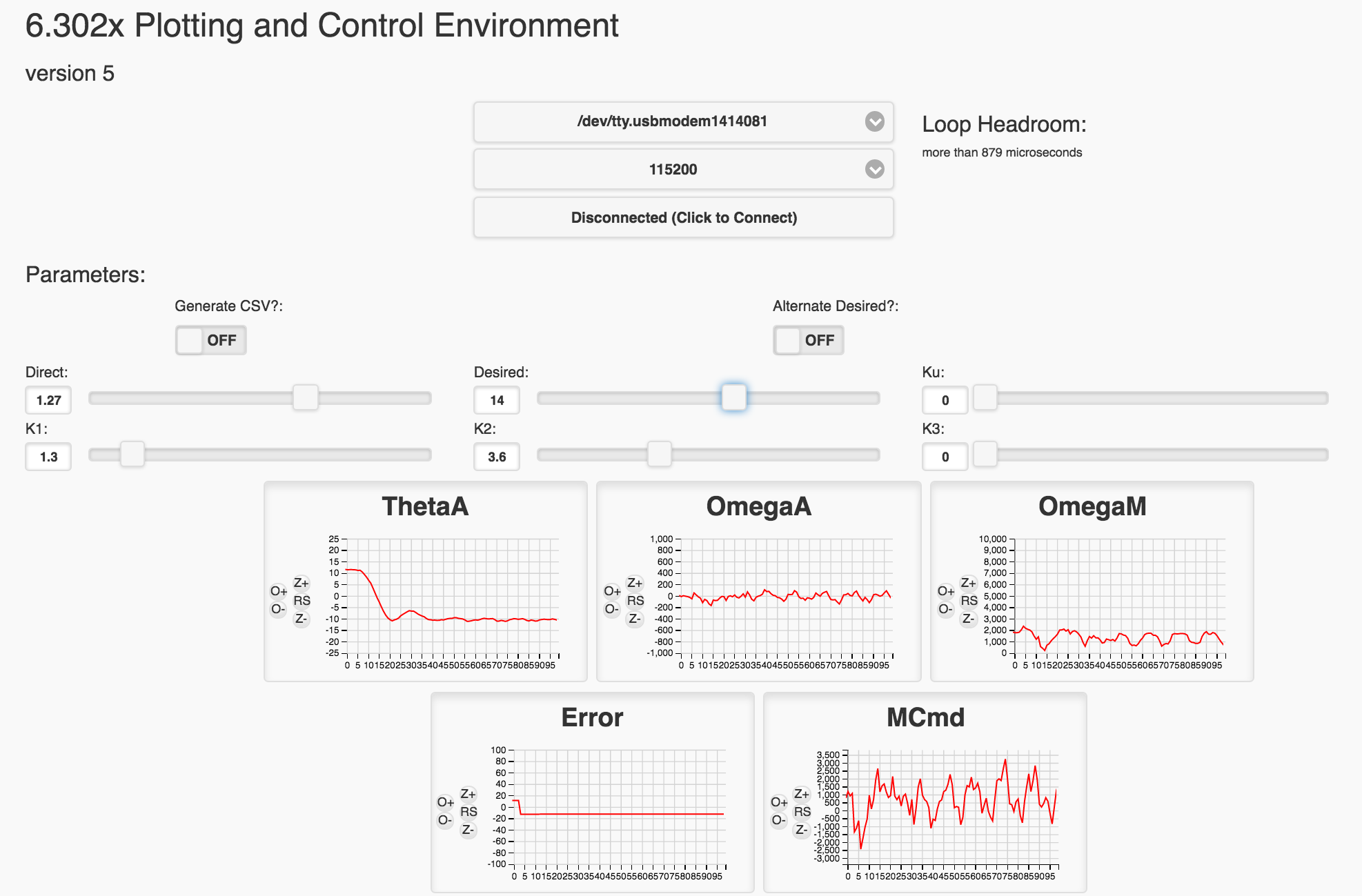
Your task for today, is to familiarize yourself with the code and implement a proportional + difference control using the state variables. When running your code GUI will ultimately look like the following:
Your task is to find the line of code that does this:
   // calculate the motor command signal here:
  float motorCmd = directV;
and modify it to implement state feedback on the arm angle. Inside the code, the \(K_1\) gain is specified as variable K1. Please keep in mind that you will have to add a term for the desired arm angle (the \( K_u \) in step feedback parlance.
The variable directV can be thought of as an offset which we'll use to cancel out the effect of gravity, and allow us to treat the system as linear about a force-balanced horizontal position. The direct term is tied to a GUI slider.
Many of our system parameters are also present:
angleV is arm angle \(\theta_a\)angleVderv is arm angular velocity\(\omega_a\)motor_omega is motor velocity \(\omega_m\)motor_bemf is the motor's back EMF \(v_{emf}\)Ku is the precompensator gain (tied to GUI slider)desiredV is the desired arm angle \(u\) (tied to slider in the GUI)You will be using these variables to implement measured-state feedback on the arm angle state, as we show in what follows. When you make changes to the Teensy code, upload it to your Teensy and then start the GUI. And whenever running an experiment, start by setting all the sliders to zero, and then adjusting the direct value so that the propeller spins fast enough to lift the arm to a little below the horizontal. Then adjust the gains for the controller you are trying to implement.
Using the browser-based GUI, and setting all other sliders set to zero, you can use the direct slider to increase the average voltage used to drive the motor for your copter-levitated arm. The higher the average voltage, the faster the propeller spins, generating more thrust to lift the arm (see figure 1 below). If your propeller is spinning the correct direction, then when you (slowly!!!) increase the direct slider, the arm will lift upwards, but if you increase the direct term too much, the arm will fly away (careful!!).
If your propeller is spinning the wrong direction, the thrust will push the arm downwards, but that is easily fixed. Just switch two jumper wires that connect the motor to the circuit board. One motor wire is connected to ground and the other motor wire is connected to one end of the half-ohm resistor, swap them and the propeller will reverse direction, reversing the thrust direction. Note that the motor wires are the thicker pair of wires from the copter, the thinner pair of wires are connected to the light emitting diode on the bottom of the copter.
Try adjusting the direct command so that the arm sits about \(45^{\circ }\) below horizontal, as in Figure 1, and then try to adjust the direct term to make the arm horizontal.
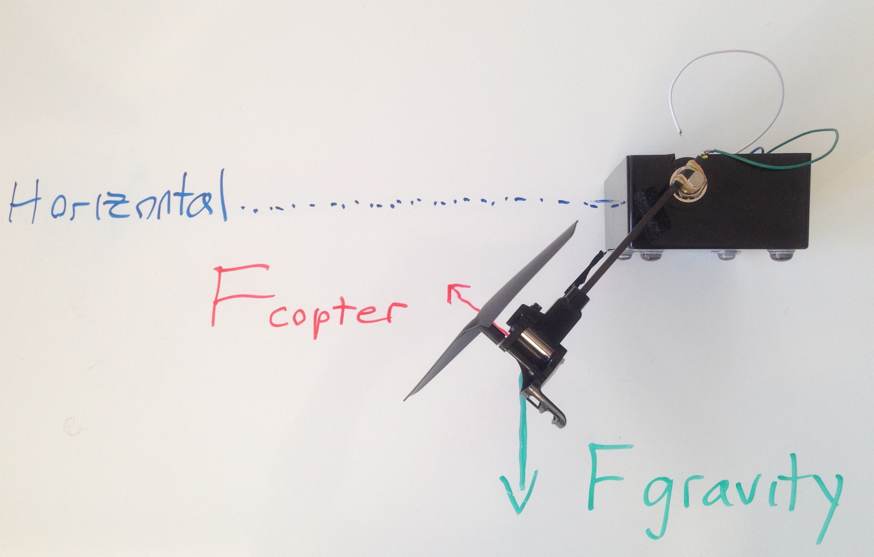
Figure 1: The arm positioned approximately \(45^{\circ }\) below horizontal. Note, picture of an earlier version of the lab hardware.
It is unlikely that you will be able to adjust the direct command so that the arm is perfectly horizontal, but you can probably get close. With the arm near horizontal, the motor thrust exactly balances the gravity force, as shown in figure 2.
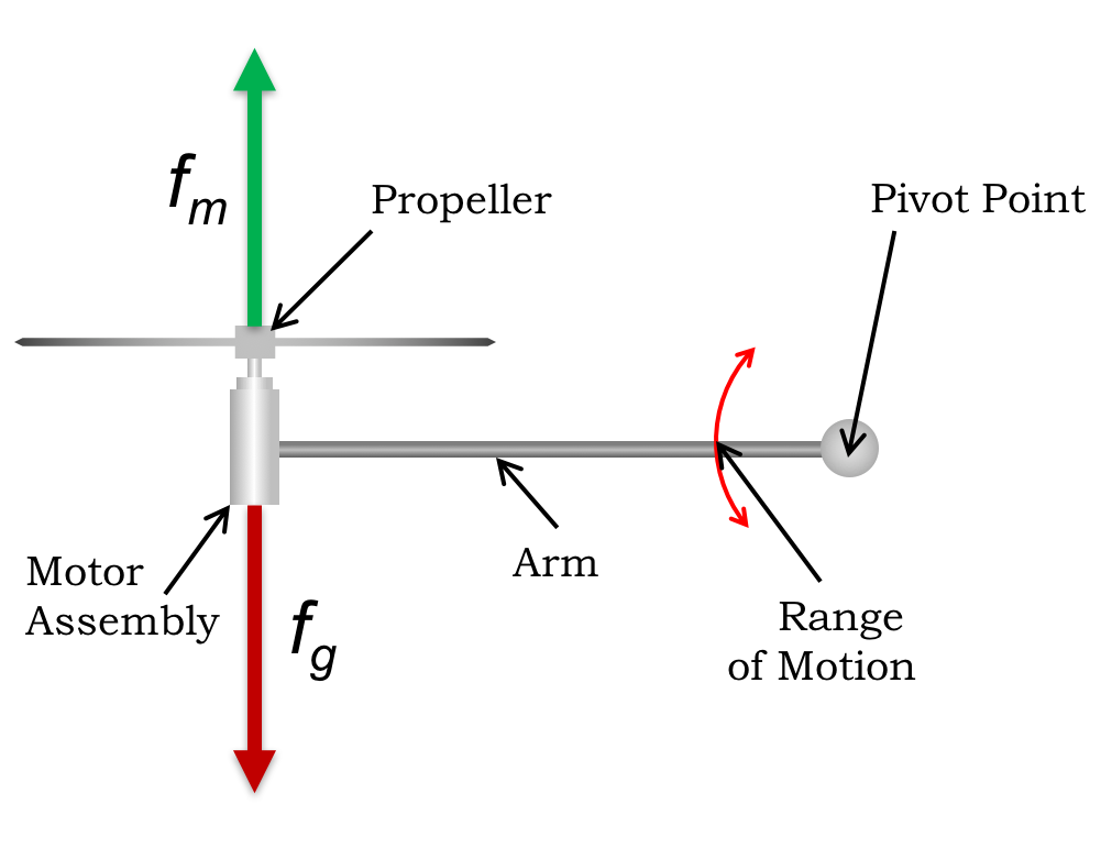
Figure 2: The horizontal arm, with the upward thrust force balancing the gravity force.
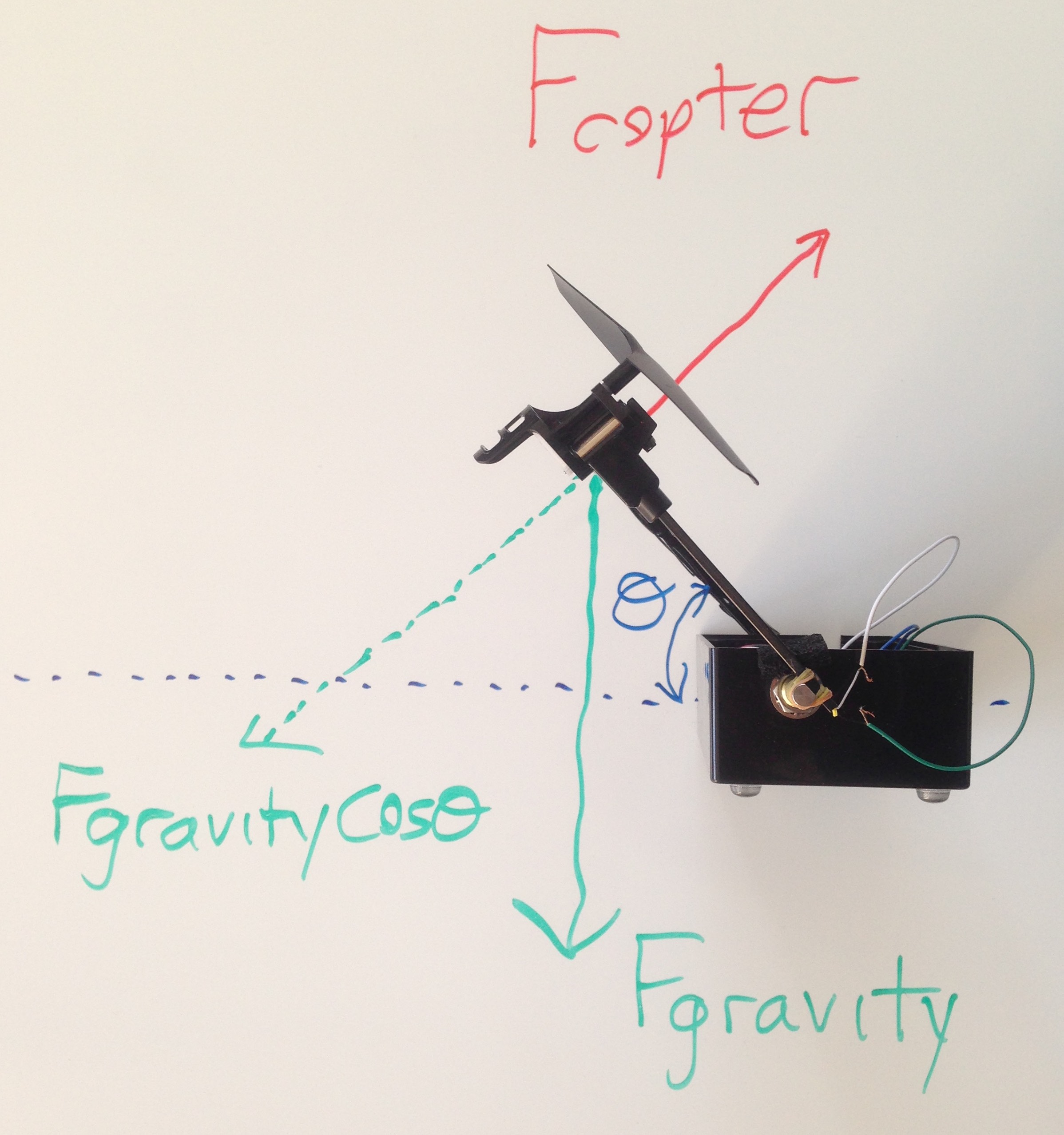
Figure 3: The arm positioned approximately \(45^{\circ }\) above horizontal.
For most of our experiments with the copter-levitated arm, we will start by adjusting the direct term to make the arm nearly horizontal with all other sliders set to zero. We do this to make the analysis easier. That is, any feedback term we introduce will increase or decrease thust on a force neutral copter, and is reasonably modeled as linear. For example, suppose we introduce proportional feedback with gain \( K_p \). On the Teensy, that would mean,
float motorCmd = directV + K1*(desiredV - angleV);
where \( desiredV \) will be desired angle, whose suitably-scaled version we will denote as \( \theta_d \), \( angleV \) will be measured arm angle, whose suitably-scaled version we will denote as \( \theta_a \). These and other notations are shown in the arm diagram in Figure 4 below.
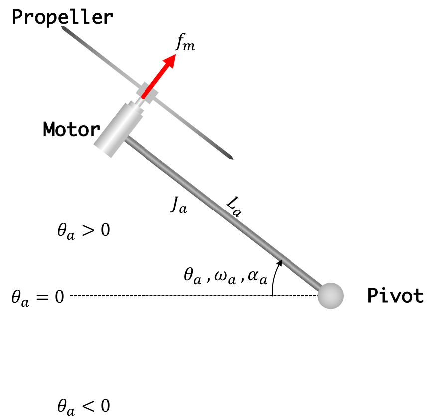
Figure 4:
Taking advantage of the fact that the direct term cancels the gravity, the net arm acceleration, \( \alpha \), will be approximately \[ \alpha \approx \gamma K_p (\theta_d - \theta_a). \] where \( K_p \) is the proportional feedback gain, \( \gamma \) is a proportionality constant one must determine by experiment (or modeling, which we will do later).
To develop a state-space model for the copter-levitated arm, we should first note that when we use a control loop on the Teensy, we are introducing a sampling interval, \(T = 0.001 \) seconds, so we will develop the state-space model in discrete time.
The angle of our propeller \(\theta_a[n]\) can be said to be based on the prior version of itself as well as the prior angular velocity \(\omega_a[n-1]\) such that: \[ \theta_a[n] = \theta_a[n-1] + T \cdot \omega_a[n-1] \]
In turn, the angular velocity of the arm \(\omega_a[n]\) is based on its prior value as well as the prior value of its angular acceleration. That is, \[ \omega_a[n] = \omega_a[n-1] + T \cdot \alpha_a[n-1]. \]
If we again assume that: the direct term cancels gravity, acceleration is produced by a feedback term, and we are using proprotional feedback, ... \[ \omega_a[n] = \omega_a[n-1] + T \cdot \alpha_a[n-1] = \omega_a[n-1] + T \cdot \gamma K_p (\theta_d[n-1] - \theta_a[n-1]). \]
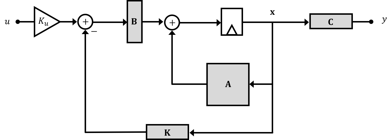
Consider converting the two state equations from the above section in to a state space model. Given the two difference equations \[ \theta_a[n] = \theta_a[n-1] + T \cdot \omega_a[n-1] \] and \[ \omega_a[n] = \omega_a[n-1] + T \cdot \gamma K_p (\theta_d[n-1] - \theta_a[n-1]), \] there is an equivalent state-space form, \[ \textbf{x}[n] = \textbf{A} \textbf{x}[n-1] + \textbf{B} \left(K_u \theta_d[n-1] - \textbf{K} \textbf{x}[n-1] \right) \] where \[ \textbf{K} = [K_1 \; K_2] \;\; \text{and} \;\; \textbf{x}[n] = \begin{bmatrix}\theta_a[n]\\ \omega_a[n]\end{bmatrix}. \] In the following questions you will determine the state-space form, and then answer questions about the the eigenvalues of the state-space model as a function of state feedback gains. These will help you determine values to use for \(K_1 \) and \(K_2 \) for your copter-levitated arm.Note: Make sure you select all of the correct options—there may be more than one!
Explanation
Look the difference equations.
Explanation
Look the difference equations.
Explanation
Look the difference equations.
Explanation
Look the difference equations.
Explanation
Look the difference equations.
Explanation
Look the difference equations.
Explanation
Look the difference equations.
Explanation
Look the difference equations.
Explanation
Look the difference equations.
We know from the notes that the feedback system involving \( \textbf{x}[n] \) is given by \[ \textbf{x}[n] = \textbf{M} x[n-1] + \textbf{B} K_{u} \theta_d[n] \] where \[ \textbf{M} = \textbf{A} - \textbf{B} \textbf{K}. \]
In addition, the eigenvalues of \( \textbf{M} \) are the natural frequencies of the feedback system, and natural frequencies tell us a lot about the behavior of a system. In the case of our two-state discrete-time model of the copter-levitated arm, \[ \textbf{M} = \begin{bmatrix} 1.0 & T\\ -T \cdot \gamma \cdot K_1 & 1.0 \end{bmatrix} \] where \( T = 0.001 \) is the Teensy sample period in seconds. The following questions refer to a copter-levitated arm where the acceleration due to the feedback term has a proportionality constant of \( \gamma = 10 \) (not a realistic value for your arm, most likely).
If the natural frequencies for the feedback system are the complex numbers \( 1 - 0.001j \) and \( 1 + 0.001j \), what is the the closest approximate value of \( K_1 \).
If the natural frequencies for the feedback system are the complex numbers \( 1 - 0.003j \) and \( 1 + 0.003j \), what is the the closest approximate value of \( K_1 \).
If the natural frequencies for the feedback system are the complex numbers \( 1 - 0.01j \) and \( 1 + 0.01j \), what is the the closest approximate value of \( K_1 \).
The natural frequencies for the feedback system, as a function of \( K_1\), are given by \( 1 - f(K_1) j \) and \( 1 + f(K_1) j \), where the function \( f \) is
For each of the following ten-second feedback system step responses, determine the proportional gain, \( K_1\).
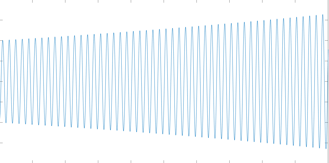
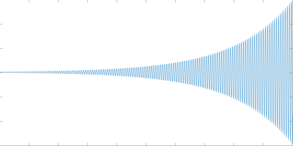
For the very oscillatory step responses of these three feedback systems, what does \( \frac{2 \pi }{|imag(\lambda_1)|}*T \) estimate? In this case, \( |imag(\lambda_1)| \) is the absolute value of the imaginary part of either eigenvalue of \( M\), and \( T = 0.001 \) is the sampling period.
For the very oscillatory step responses of these three feedback systems, what does \( |\lambda_1|^{100000} \) estimate? In this case, \( |\lambda_1| \) is the magnitude of either eigenvalue of \( M\), and \( T = 0.001 \) is the sampling period.
In this problem you will try using proportional control with your arm, and if your arm is like ours, for very small proportional gains, the arm is stable and you can position it to be nearly perfectly horizontal. Based on your numbers, you will try to determine a value for \( \gamma \), described above, and a value for a friction parameter \( \beta \), described below, for a two-state model of your arm.
Since our two-state model is not stable for ANY positive value of \( K_1 \), but the arm is stable for small gains, something is missing. One possibility is that friction decelerates the arm, so the form of a linear friction term in the acceleration equation would be \[ -\beta \omega_a[n]. \]
Where does \( \beta \) go in the feedback system matrix \( \textbf{M} \)? And should it be scaled by the sampling period \(T?\)
What was the largest value of \( K_1 \) you could use and still have the arm be stable?
What value did you use for \( \beta \) in your two-state model?
What value did you use for \( \gamma \)?
In this experiment you will try using proportional control with your arm, and if your arm is like ours, very small proportional gains will stabilize the arm enough that it can hold a perfectly horizontal position. Then you will examine the two-state model from the previous section, to see if it predicts the stability of the arm with low proportional gain (spoiler alert, it does not). You will then try to add linear friction to your model, to see if the model can better predict your experiment (it can). And finally, you will try to think up an experiment or two to help you calibrate your model, and then report your findings.
float motorCmd = directV + K1*(desiredV - angleV);
We derived a state-space representation for our two-state model of the propeller arm with proportional feedback, \[ \textbf{x}[n] = \textbf{M} x[n-1] + \textbf{B} K_{u} \theta_d[n] \] where \[ \textbf{M} = \textbf{A} - \textbf{B} \textbf{K} = \begin{bmatrix} 1.0 & T\\ -T \cdot \gamma \cdot K_1 & 1.0 \end{bmatrix} \] where \( T = 0.001 \) is the Teensy sample period in seconds
The eigenvalues of \( \textbf{M} \) are the natural frequencies of the feedback system, and for the feedback system to be stable, the natural frequencies must have magnitudes less than one. Our experiment showed that the arm is stable for small values of \( K_1 \), but it is easy to show that for the model above, both eigenvalues of \( \textbf{M} \) have magnitudes greater than one FOR ALL POSTIVE VALUES of \(K_1\).
Such a significant inconsistency between model and experiment usually means something is missing from the model, and in this case, the culprit is probably rotational friction. To add linear rotation friction term to the rotational acceleration equation is straight-forward, but if we model it phenomenologically, we will need another coefficient. Specifically, the rotational acceleration due to rotational friction could be represented as \[ - \beta \omega_a \] where \( \beta \) is the friction coefficient, and the negative sign indicates that friction decelerates the arm.
Using the friction term, the update equation for \( \omega_a \) becomes \[ \omega_a[n] = \omega_a[n-1] + T \cdot \gamma K_p (\theta_d[n-1] - \theta_a[n-1]) - T \cdot \beta \omega_a[n-1]. \] and can be added to \( \textbf{M} \) as in \[ \textbf{M} = \textbf{A} - \textbf{B} \textbf{K} = \begin{bmatrix} 1.0 & T\\ -T \cdot \gamma \cdot K_1 & 1.0 - T \cdot \beta \end{bmatrix} \]
As a final step, try to determine values for two parameters in your model:
In this problem you will try using proportional control with your arm, and if your arm is like ours, for very small proportional gains, the arm is stable and you can position it to be nearly perfectly horizontal. Based on your numbers, you will try to determine a value for \( \gamma \), described above, and a value for a friction parameter \( \beta \), described below, for a two-state model of your arm.
What was the largest value of \( K_1 \) you could use and still have the arm be stable?
What value did you determine for \( \beta \) in your two-state model?
What value did you determine for \( \gamma \)?
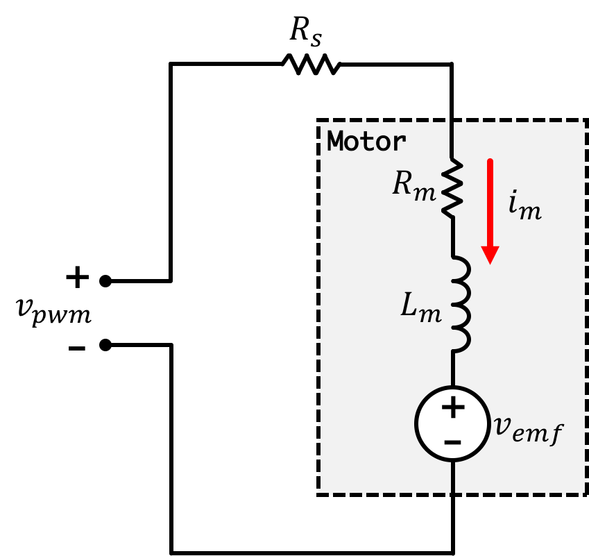
Let's start off thinking about our motor. A motor can be modeled as a series resistance \(R_m\), an inductor \(L_m\), and voltage source representing the Back EMF (electromotive force), \(v_{emf}\), with a current \(i_m\) flowing through it. Electrically speaking in our system, we can draw up the following schematic where \(v_{pwm}\) is our applied voltage and \(R_s\) is a series resistance (in our case the big green 0.5 Ohm resistor):
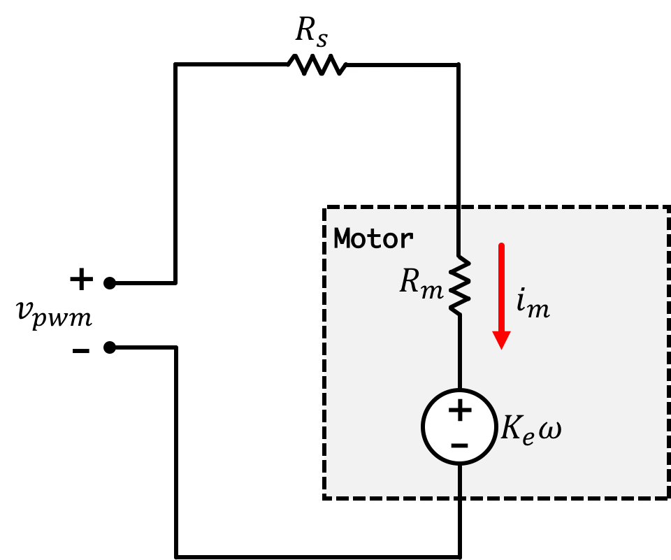
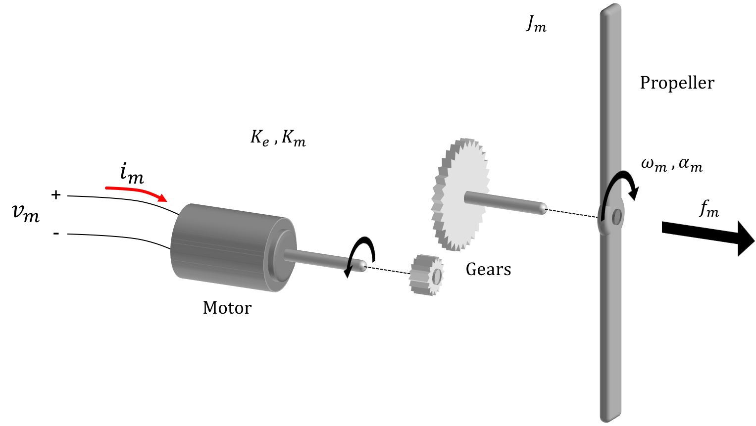
Now motor torque \(\tau_m\) can be expressed as the product of motor current and a motor torque coefficient \(K_m\): \[ \tau_m(t) = K_mi_m(t) \] Acceleration of the motor from \(\alpha_m\) is derived from motor torque and the motor's moment of inertia \(J_m\): \[ \tau_m(t) = J_m\alpha_m(t) \] or rearranged with : \[ \alpha_m(t) = \frac{K_m\left(v_{pwm}(t) - K_e\omega_m(t)\right)}{J_m\left(R_m+R_s\right)} \] If we then add a friction term corresponding to motor angular velocity, where \(K_f\) is a friction coefficient we get: \[ \alpha_m(t) =\frac{d\omega_m(t)}{dt}= \frac{K_m\left(v_{pwm}(t) - K_e\omega_m(t)\right)}{J_m\left(R_m+R_s\right)}-K_f\omega_m(t) \]
In 6.302.1x, we're more focussed on discrete time models, so we can convert this continuous time (\(t\)) equation into a discrete time form, so converting this into a discrete time equivalent we end up with: \[ \frac{d\omega_m(t)}{dt} \approx \frac{\omega_m[n]-\omega_m[n-1]}{T} = \frac{K_m\left(v_{pwm}[n-1] - K_e\omega_m[n-1]\right)}{J_m\left(R_m+R_s\right)}-K_f\omega_m[n-1] \] and we can rewrite this so: \[ \omega_m[n] = \left(1-\frac{TK_mK_e}{J_m\left(R_m+R_s\right)}-TK_f\right)\omega_m[n-1] + \frac{TK_m}{J_m\left(R_m+R_s\right)}v_{pwm}[n-1] \]
In turn, the angular velocity of the arm \(\omega_a[n]\) is based on its prior value as well as the prior value of angular acceleration of the arm multiplied by the timestep. For now to linearize the system, we will assume the only force working on the system is that from the propeller. A general equation would be: \[ \omega_a[n] = \omega_a[n-1] + T\alpha_a[n-1] \] The angular acceleration is based off of the torque on the arm \(\tau_a\) divided by the moment of the arm \(J_a\): \[ \alpha_a[n]=\frac{\tau_a[n]}{J_a} \] The torque in on our arm is based on the cross product of the thrust \(f_m\) from the propeller and the length of the propeller arm \(L_a\). \[ \tau_a[n] = L_a\times f_m[n] \] Since these two are at right angles to one another we can simply say: \[ \tau_a[n] = L_af_m[n] \] All together therefore, we can say that: \[ \alpha_a[n] = \frac{L_af_m[n]}{J_a} \]
We've found through the data collection that the thrust from the propeller can be approximated as being linearly proportional to motor speed such that: \[ f_m[n] = K_t\omega[n] \] Reorganizing this we end up with: \[ \omega_a[n] = \omega_a[n-1] -\frac{TK_tL_a}{J_a}\omega_m[n-1] \]
We've now filled in three equations which we can use to construct our state space matrices: \[ \theta_a[n] = \theta_a[n-1] +T\omega_a[n-1] \] and \[ \omega_a[n] = \omega_a[n-1] +\frac{TK_tL_a}{J_a}\omega_m[n-1] \] and \[ \omega_m[n] = \left(1-\frac{T K_mK_e}{J_m\left(R_m+R_s\right)}-T K_f\right)\omega_m[n-1] + \frac{T K_m}{J_m\left(R_m+R_s\right)}v_{pwm}[n-1] \] \[ \begin{bmatrix} \theta_a[n] \\ \omega_a[n]\\ \omega_m[n]\\ \end{bmatrix} = \begin{bmatrix} 1 & T & 0\\ 0 & 1 & \frac{TK_tL_a}{J_a}\\ 0 & 0 &\left(1-\frac{TK_mK_e}{J_m\left(R_m+R_s\right)}-TK_f\right)\\ \end{bmatrix} \begin{bmatrix} \theta_a[n-1] \\ \omega_a[n-1]\\ \omega_m[n-1]\\ \end{bmatrix} + \begin{bmatrix} 0\\ 0 \\ \frac{TK_m}{J_m\left(R_m+R_s\right)} \\ \end{bmatrix}v_{pwm}[n-1] \] and also: \[ y = \begin{bmatrix}1 & 0 & 0\\ \end{bmatrix} \begin{bmatrix} \theta_a[n] \\ \omega_a[n]\\ \omega_m[n]\\ \end{bmatrix} \]
While we'll investigate modeling significantly more in Week 2 in 6.302.1x, it wouldn't be bad to start sticking numbers to some of the constants we've been using in our derivations and modeling.
Starting with the derived \(\textbf{A}\) matrix above representing our plant we can label the individual elements in it as follows:\[ \textbf{A} = \begin{bmatrix}a_{11} & a_{12} & a_{13}\\ a_{21} & a_{22} & a_{23}\\ a_{31} & a_{32} & a_{33}\\ \end{bmatrix} \] If we wanted to implement a rotational friction/drag coefficient on the arm, what term would we modify?
Explanation
\(a_{22}\) corresponds to the influence of past arm angular velocity to current arm angluar velocity. Friction in a rotational frame of reference can be described as force opposing the current velocity such that \(f_{friction}[n] = K_{fa}\omega_a[n]\) and since force will result in an direct influence on angular acceleration \(\alpha_a[n]\) of the arm we could rewrite our second equation from above as: \[ \omega_a[n] = \omega_a[n-1] -\frac{TK_{fa}L_a}{J_a}\omega_a[n-1] + \frac{TK_tL_a}{J_a}\omega_m[n-1] \]
With your propeller running with no feedback (just a low constant fixed voltage on the motor), if you were to quickly move the arm up or down (using your hand) you should notice (via the tone of the motor) that the motor speed is varying because of the forcing of more or less air through the propeller (varying the drag on the prop). How could we implement this phenomenon in our state space model?
Starting with the derived \(\textbf{A}\) matrix above representing our plant we can label the individual elements in it as follows:\[ \textbf{A} = \begin{bmatrix}a_{11} & a_{12} & a_{13}\\ a_{21} & a_{22} & a_{23}\\ a_{31} & a_{32} & a_{33}\\ \end{bmatrix} \] If we wanted to add in a term capturing the phenomenon what term would we modify?
Explanation
\(a_{32}\) corresponds to the influence of arm velocity on motor velocity. That is the correct set of parameters altered in the phenomenon described above.
In what way would the presence of drag modify the \(\textbf{A}\) matrix parameter you chose above?
Explanation
The change in \(a_{32}\) can be thought about as follows: When the propeller is moving upwards (positive angular velocity of the arm), we are helping the prop out, making it need to fight the air a little bit less...this decrease in opposition force will correspond to a slightly higher speed. Alternatively when the prop arm is being turned downwards, we can think of it as having more air being shoved up through the blades, giving it a harder time...In both situations, a positive term for \(a_{32}\) would express this (the exact value is of course up for speculation/experimentation). I'll call this variable \(K_d\) for now and we'll simply say \(K_d > 0\):
\[ \begin{bmatrix} 1 & T & 0\\ 0 & 1 & \frac{TK_tL_a}{J_a}\\ 0 & K_d &\left(1-\frac{K_mK_e}{J_m\left(R_m+R_s\right)}-K_f\right)\\ \end{bmatrix} \]Based on what we discussed in the notes, while our propeller arm system has a plant expressed with the matrices derived on the previous page (of which the eigenvalues of the \(\textbf{A}\) matrix are its natural frequencies) , we can use state feedback in order to modify those eigenvalues towards the goal of stabilizing the system:
For Week 1, we're just going to roughly gauge numbers to pick based on experience in 6.302.0x. In Week 2, we'll look at more quantitative ways of assigning the feedback gains.
Starting with \[ \textbf{K} = \begin{bmatrix}K_1\\K_2\\K_3\end{bmatrix}=\begin{bmatrix}0\\0\\0\end{bmatrix} \] If we wanted to implement proportional only control on the arm angle, what term would we adjust and how would we do it?
Explanation
\(K_1\) is directly multiplied by the \(\theta_a\) state, and because we subtract the result of \(\textbf{K}\cdot\textbf{x}[n-1]\) we'd want a positive value fo \(K_1\) to implement proportional control. This will only make sense, however, if \(K_u\) is adjusted appropriately!
When carrying out Proportional + Derivative Control (a PD controller), a gain \(K_d\) is applied to the derivative of the error signal. In the case of state feedback to control the arm angle in our propeller setup, what value of the \(\textbf{K}\) matrix would need to be changed (and how) in order to implement derivative control?
Starting with \[ \textbf{K} = \begin{bmatrix}K_1\\K_2\\K_3\end{bmatrix}=\begin{bmatrix}0\\0\\0\end{bmatrix} \] If we wanted to implement proportional+Derivative control on the arm angle, what term would we adjust and how would we do it?
Explanation
\(K_2\) is directly multiplied by the \(\omega_a\) state, and because we subtract the result of \(\textbf{K}\cdot\textbf{x}[n-1]\) we'd want a positive value fo \(K_2\) to implement proportional control.
When carrying out Proportional + Derivative Control (a PD controller), a gain \(K_d\) is applied to the derivative of the error signal. Assuming our input stays constant, and building upon your answer above, would we need to modify \(K_u\) in order to properly implement true discrete time derivative control in our system (in conjunction with the change you stated in the situation above?)
Explanation
To quickly do a continuous time analysis we can say our error is: \[e(t) = \theta_d(t) - \theta_a(t)\] if our input (desired angle) stays relatively constant with time, then when we take the time derivative of our error we'd get: \[\frac{de(t)}{dt} \approx \frac{\theta_a(t)}{dt} \] Since one of our states is \[ \omega_a = \frac{\theta_a(t)}{dt} \] that means applying a gain onto the the system's angular velocity (gain \(K_2\)) will be the same! No modification of \(K_u\) is necessary in order to make sure derivative control is implemented!
When carrying out Proportional Control (a P controller), a gain \(K_p\) is applied to the error signal. Assuming our input stays constant, and building upon your answer above, would we need to modify \(K_u\) in order to properly implement proportional control in our system (in conjunction with the change you stated in the situation above?)
Explanation
Yes in Proportional control we drive our plant with \(K_p\) times an error signal. In the situation of our system, our error is defined as: \[ e[n] = \theta_a[n] - u[n] \] For us to implement true proportional control we need to drive our plant with: \[ K_pe[n] \] For that to be true, the signal going into our plant must be: \[ input_[n] = K_p\left(\theta_a[n] - u[n]\right) \] As discussed above, a positive \(K_1\) will take care of part of the proportional gain implementation, but it will not take care of the \(K_p\theta_a[n]\) term, so we need to also have \(K_u = K_p\) in order to implement proportional control fully.
If you'd like, using sympy or another symbolic matrix library, calculate \(K_u\) out officially using our expression for it below:
\[
K_u = \left(\textbf{C}\left(\textbf{I}-\textbf{A}+\textbf{BK}\right)^{-1}\textbf{B}\right)^{-1}
\]
If you coded up/implemented all of your matrices properly, you should get the same value for \(K_u\) as we reasoned through in the question above (see solutions on this page!). We can discuss this more in the forum as needed! This is a good sanity check that you are implementing your state space model appropriately in code if you're doing that!
Can we design a better position controller using state feedback with all the states, not just the arm angle? For this experiment you are going to try, but you will find that we really do not have the tools to find the best values for the \(K_i's\), but perhaps you can find pretty good ones. And in addition, you will encounter a problem with scaling variables, an important practical matter.
Recall that running your code GUI will look like the following:
Your task is to find the line of code that does this:
   // calculate the motor command signal here:
  float motorCmd = directV;
and modify it to implement state feedback on all three states. Inside the code the three \(\textbf{K}\) gain matrix parameters are specified as variables K1, K2, and K3 (tied to sliders)
The variable directV can be thought of as an offset which we'll use to cancel gravity out, as well as sort of compensate for other linearizations that we undertook. It is tied to a GUI slider.
Many of our system parameters are also prsent:
angleV is arm angle \(\theta_a\)angleVderv is arm angular velocity\(\omega_a\)motor_omega is motor velocity \(\omega_m\)motor_bemf is the motor's back EMF \(v_{emf}\)Ku is the precompensator gain (tied to GUI slider)desiredV is the input signal \(u\) (tied to slider in the GUI)You will be using these variables to implement measured-state feedback on the states we will discussing in what follows. When you make changes to the Teensy code, upload it to your Teensy and then start the GUI. And whenever running an experiment, start by setting all the sliders to zero, and then adjusting the direct value so that the propeller spins fast enough to lift the arm to a little below the horizontal. Then adjust the various gains for the controller you are trying to implement.
Once you have a stable operating system from adjusting the direct offset term as well as \(K_1\) and \(K_2\) and \(K_u\), add in some gain on the \(K_3\) term. You should notice the system completely stop running even for extremely low values (\(K_3 = 0.1\)). In fact you should see it start to obtain a periodic burst activity Why is this?
Explanation
While both \(\theta_a\) and \(omega_a\) remain relatively small in value during normal operation (check your plots!), the motor speed (measured in radians per second) is rather large numerically (again check your plot). Consequently when we apply even a small amount of gain to the motor speed state, (relative to what we're doing with \(K_1\) and \(K_2\) the resulting signal is very negative. This isn't saying we can't utilize the \(\omega_m\) state for feedback, rather the gain we apply to it must be even smaller than what we're thinking. We must think of another way to represent that state.
One way to fix this scaling issue is to replace our motor speed state variable \(\omega_m\) with the back EMF voltage (\(K_e\omega_m = v_{emf}\). This has two advantages:
When combined, these two features mean this signal could be a more readable state, and when we really pursue proper full-state feedback in Lab 2 this will be the state we use, however we will come back to the implications of differences in signal/state units during that discussion.
In order to work with this new state, we need to modify our state space model a bit by replacing and adjusting the third row (corresponding to the motor velocity state) as well as any states which it modifies. This will result in changes to matrix of the state vector as well as \(\textbf{A}\) matrix value \(a_{23}\) to "undo" the new \(K_e\) implied in the state as well as the the \(b_{31}\) term of \(\textbf{B}\) matrix: \[ \begin{bmatrix} \theta_a[n] \\ \omega_a[n]\\ K_e\omega_m[n]\\ \end{bmatrix} = \begin{bmatrix} 1 & T & 0\\ 0 & 1 & \frac{TK_tL_a}{K_eJ_a}\\ 0 & 0 &\left(1-\frac{TK_mK_e}{J_m\left(R_m+R_s\right)}-TK_f\right)\\ \end{bmatrix} \begin{bmatrix} \theta_a[n-1] \\ \omega_a[n-1]\\ K_e\omega_m[n-1]\\ \end{bmatrix} + \begin{bmatrix} 0\\ 0 \\ \frac{TK_eK_m}{J_m\left(R_m+R_s\right)} \\ \end{bmatrix}v_{pwm}[n-1] \] and also the following, although since we don't use that third state in our output it doesn't change from before much. \[ y = \begin{bmatrix}1 & 0 & 0\\ \end{bmatrix} \begin{bmatrix} \theta_a[n] \\ \omega_a[n]\\ K_e\omega_m[n]\\ \end{bmatrix} \]
Change the motor speed state you're currently using to apply a gain in the to the back emf instead. To modify your code replace the line at the top of the code that says String config_message_lab_1_6302d1 = with the following (this adjusts the plots to expect/label for Back EMF and not Omega
String config_message_lab_1_6302d1 = "&A~Desired~5&C&S~Direct~O~0~2~0.01&S~Desired~A~-90~90~1&S~Ku~U~0~10~0.01&S~K1~B~0~10~0.01&S~K2~C~-0~10~0.01&S~K3~D~-0~10~0.01&T~ThetaA~F4~-100~100&T~OmegaA~F4~-1000~1000&T~Vemf~F4~0~5&T~Error~F4~-100~100&T~MCmd~F4~0~5&D~100&H~4&";And change the line:
packStatus(buf, angleV*rad2deg, angleVderv*rad2deg, motor_omega, errorV*rad2deg, motorCmdLim, float(headroom));So that it says the following (reporting motor back EMF rather than motor velocity \(\omega_m\)):
packStatus(buf, angleV*rad2deg, angleVderv*rad2deg, motor_bemf, errorV*rad2deg, motorCmdLim, float(headroom));
Reload the code onto the microcontroller, restart the server (press control C if you don't know how), and then restart. Addition of a bit of gain on the third state now, while not necessarily giving a much improved response, is at least not completely removing the command signal now!